Sediment Accumulation Rates and High-Resolution Age-Depth Models

INTRODUCTION

One of the key goals of most sedimentological studies is to understand the depositional environment. Sediment accumulation rates–the net accrual of sediment over time accounting for deposition, erosion, and tectonism–offer insight into paleoenvironment interpretations and reflect trends in accommodation and sediment supply (e.g., Reading, 2009). As a result, stratigraphers have worked to better understand sediment accumulation processes for over a century. Two of the most significant advancements in this field were the establishment of an inverse relationship between timespan and accumulation rate and, subsequently, the demonstration that stratigraphic completeness deteriorates with timespan (this phenomenon is referred to as the Sadler Effect; Schumer & Jerolmack, 2009). Stratigraphic completeness is typically reported for a specific timespan as a percentage; for example, stratigraphic completeness could be described as 75% at 1-Myr intervals for a given stratigraphic record, meaning that three out of every four 1-Myr intervals of time are represented by at least some rock (Sadler, 1981). This relationship is best viewed on log-log plots, which are colloquially referred to as Sadler plots. Note that while this mathematical approach to understanding sediment accumulation can offer powerful insights, field observations and sedimentological descriptions are still necessary to fully understand the depositional history of a given stratigraphic record. In addition, there has been discussion regarding whether “completeness” is an appropriate term (Miall & Hessler, 2024); I continue to use the term in this contribution as no alternative has been proposed and accepted by the community, and stratigraphic completeness clearly represents a real and useful metric for stratigraphers (e.g., Miall, 2016; Paola et al., 2018; Sadler, 1981).

Due to the fractal nature of sediment accumulation, the relationship between accumulation rate and duration is a negative power law (Sadler, 1999). This negative power law, while sometimes related to depositional setting, is largely the result of randomness (Schumer et al., 2011; although cyclicity is also often observed; Sadler, 1994). The stochastic nature of sediment transport and accumulation is an area of active research with important implications for the interpretation of climate archives (e.g., Jerolmack, 2009, 2011; Phillips & Jerolmack, 2016). Further complicating stratigraphic interpretations, depositional environment can have a strong control on estimated stratigraphic completeness. For example, Holocene tidal estuary estimates range from ~20–48% complete versus Holocene sediment-starved slope estimates of ~85–100% complete (Sommerfield, 2006). What has emerged from this literature is a narrative that is broadly true–that a negative power law defines the relationship between accumulation rate and duration–but has some complicating aspects and could use further refinement.

Historically, researchers have used large data compilations, which pool together broad accumulation rate data, to establish the above relationships. New advances in geochronologic and age modeling techniques have enabled high-resolution age-depth models for stratigraphy. For example, Bchron uses a Bayesian statistics approach to create continuous age-depth models from discrete geochronologic dates, thereby estimating a mean age with uncertainty for each horizon (see Haslett & Parnell, 2008; Parnell, 2014). Note that in this contribution I do not use “horizon” in the strict traditional sense from field geology; instead, I use “horizon” to broadly mean a discrete dated instance, which includes dated “horizons” in synthetic age-depth models as well as dated carbon isotope values in Ediacaran composite records (see Hagen & Creveling, 2024).

While researchers have shown that the relationships put forward in Sadler (1981) can be found in larger data compilations (e.g., Kemp & Sadler, 2014), similar assessments have not often been made for individual stratigraphic records that have a high-resolution age-depth model. While many previous contributions have investigated accumulation rate–duration trends and the Sadler Effect using both large-scale compilations and individual stratigraphic records (e.g., Aadland et al., 2018; Anders et al., 1987; Sadler, 1999; Sadler & Jerolmack, 2015; Sadler & Strauss, 1990; Strauss & Sadler, 1989), it is my aim to build on this body of important work.

In this contribution, I explore the Sadler Effect in, and Sadler plots generated from, individual stratigraphic records with high-resolution age-depth models (in this case, Bayesian-based age models with age estimates, and uncertainty, for every individual horizon in the stratigraphic record). First, I create simplified, synthetic high-resolution age-depth models and demonstrate how to extract a sufficient dataset from individual records. I then apply this approach to regional composite stratigraphic records from the Ediacaran Period as a test case. I demonstrate how this Sadler plot approach can be applied to real datasets representing individual stratigraphic sections and can yield key insights into local-regional depositional histories.

METHODOLOGY

Sediment accumulation rates and stratigraphic completeness

Sediment accumulation rates are classically calculated between two horizons, i (overlying) and j (underlying), with geochronologic age constraints, where the accumulation rate, s, is simply the difference in stratigraphic height, H, over the difference in age, T:

$$s_{i,j} = \frac{H_{i} - H_{j}}{T_{j} - T_{i}}$$

In this equation, the denominator serves as the time span between the two horizons (the total duration), which can be written as $d_{i,j}$ (note that at the scale of individual particle deposition, $d_{i,j}$ could go to 0).

With the advent of high-resolution age-depth models, it is possible to estimate an age for every horizon in a stratigraphic sequence. All age-depth model techniques have underlying assumptions that may influence the resulting completeness estimates; while an in-depth investigation into these assumptions is beyond the scope of this contribution, it will be the subject of future work. Using this horizon-level data, I leverage an iterative technique, where, for every horizon, i, I calculate accumulation rates and durations for each pairing of that horizon and every horizon below it (Figure 1). I store the resulting triangular matrices as vectors of accumulation rates, S, and duration, D:

$$S\, = \,\begin{matrix} \begin{matrix} \ldots \\ s_{i,i - 1} \\ s_{i,i - 2} \\ s_{i,i - n} \\ \ldots \end{matrix} \end{matrix}$$

$$D\, = \,\begin{matrix} \begin{matrix} \ldots \\ d_{i,i - 1} \\ d_{i,i - 2} \\ d_{i,i - n} \\ \ldots \end{matrix} \end{matrix}$$

Figure 1.Three synthetic high-resolution age-depth models from which iterative sediment accumulation rates were calculated.

Synthetic record 1 (A) is a linear age model, with the zoom-in schematic indicating how iterative short-term (S_short) and long-term (S_long) accumulation rates are calculated (height and age variables are colored according to stratigraphic horizon). Synthetic record 2 (B, left) is a linear age model with randomized horizon thickness, while synthetic record 3 (B, right) is a logarithmic age model (see Methodology for a more detailed description). In the synthetic records, red dashed lines indicate synthetic geochronologic constraints used in age model construction (synthetic record 3 has the same bounding ages but neither of the intervening ages).

Through this approach, I calculate accumulation rate and duration for every possible stratal pairing in the stratigraphic record, generating full distributions of calculated accumulation rates and durations for the record. This approach is very similar to how some accumulation rates and durations are calculated in existing accumulation rate databases (e.g., Kemp et al., 2020; Sadler, 1981).

Using these resulting data, I then calculate accumulation rate gradients for each record by fitting negative power law functions to the data in the accumulation rate (S) and duration (D) vectors. With these calculated gradients, I estimate stratigraphic completeness, C, using the following equation described in Sadler (1981) and pioneered by Reineck (1960):

$$C = {(\frac{t_{*}}{t})}^{- m}\tag{2}$$

where t_* is the time interval over which completeness is estimated, t is the total time interval of the record, and m is the exponential constant, or gradient, that characterizes the relationship between sediment accumulation rate and duration (larger m values result from steeper power law relationships between accumulation rate and duration, equivalent to a steeper linear slope in log-log space). For example, a record with a total duration of 20 Myr (t), assessed for completeness at a 5 Myr scale $(t_{*})$ and characterized by an accumulation rate gradient of -0.3 (m), would have an estimated fractional completeness (C) of: ${(\frac{5}{20})}^{- ( - 0.3)} = \sim 0.66$. These fitting routines are conducted on the entire suite of computed accumulation rates and durations; plots of all fitted power laws for this contribution are available in Supplementary Figures 1 and 2. I calculate two specific completeness metrics for a point of comparison between different age-depth models: the 1-Myr completeness, which is the estimated completeness (in percent) for a 1-Myr interval (setting $t_{*} = 1$ Myr and solving for C); and the 50% interval, which is the estimated interval at which the stratigraphic completeness is 50% (setting C = 0.5 and solving for $t_{*}$). Both metrics were chosen arbitrarily with the thinking that many stratigraphers would be interested in completeness at the 1-Myr interval and the required interval to ensure that at least 50% of time is captured in the rock record; a stratigrapher using this approach could easily adopt different completeness metrics of their choosing.

Synthetic age-depth models

Three simplified synthetic age-depth models serve to demonstrate my approach for calculating accumulation rates and producing iterative Sadler plots (see below) from individual stratigraphic records with high-resolution stratigraphic age models (Figure 1). These age-depth models include: a linear age-depth model; a linear age-depth model with randomized horizon thickness; and a logarithmic age-depth model. The bounding ages of each of these synthetic age models are set at 530 Ma (at 0 m) and 518 Ma (at 100 m), respectively (dashed red lines in Figure 1). The two linear age models have additional age tie points at 33 m and 67 m (525 Ma and 519 Ma, respectively; dashed red lines in Figure 1), allowing me to introduce a step-change in the accumulation rate at 67 m (see Figure 1). The logarithmic age model is calculated simply using the youngest age constraint (530 Ma at 0 m), resulting in a smoothly changing accumulation rate over time (see Figure 1). Note that these age and height assignments are arbitrary, chosen solely to generate these relatively simple synthetic age-depth models for comparison. While simple age models like these risk misestimating accumulation rates (being too unrealistic or simplistic to simulate natural accumulation; Barefoot et al., 2023), I use these age models simply to demonstrate this approach for understanding sediment accumulation rates from high resolution age-depth models (Figure 2). To better capture realistic accumulation trends, I also modify each of these three synthetic records by adding unconformities (either one 5-Myr unconformity or three 2-Myr conformities; Supplementary Figure 3) and explore the impact on the resulting Sadler plots and completeness estimates (Figure 3).

Figure 2.Sadler plots and stratigraphic completeness estimates for the three synthetic high-resolution age-depth models.

A, each data point in the Sadler plots is color-coded according to the overlying age of the two horizons used to calculate the given accumulation rate-duration pairing. In the case of synthetic records 1 and 2, there is a lot of overlap in accumulation rate–duration space over the section such that most of the data from lower in these sections (older overlying ages with warmer colors) are obscured by data from higher in the sections (younger overlying ages with cooler colors). White dots are used to indicate inflection and knickpoints referred to in the text. Green lines highlight specific contours that migrate across the accumulation rate–duration space moving up-section. B, completeness plots that display fairly similar trends across these three records, which is not surprising since each synthetic age-depth model is the same height (100 m) and all are high-resolution. Horizontal red dashed lines indicate the stratigraphic completeness at an interval of 1 Myr. Vertical red dashed lines indicate the interval corresponding to 50% stratigraphic completeness.

Figure 3.Sadler plots and stratigraphic completeness estimates for two of the synthetic high-resolution age-depth models with unconformities present.

A–B, Sadler plots color-coded according to the overlying age of the two horizons used to calculate the given accumulation rate–duration pairing for synthetic record 1 with one 5-Myr unconformity (A) and three 2-Myr unconformities (B). The impact of these unconformities on the resulting Sadler plots can be seen when compared with Figure 2A (see arrows and annotations). C, the resulting completeness estimates for synthetic record 1, demonstrating how an increasing amount of missing time (unconformities) leads to lower completeness (see black arrows). D–E, Sadler plots as in A–B for synthetic record 3 with one 5-Myr unconformity (D) and three 2-Myr unconformities (E). F, the resulting completeness estimates for synthetic record 3, depicting how greater missing time results in lower completeness (see black arrows). Horizontal color-coded dashed lines in C and F indicate stratigraphic completeness at an interval of 1 Myr while vertical color-coded dashes lines indicate the interval corresponding to 50% stratigraphic completeness. Abbreviations are as follows: accum. = accumulation; unc. = unconformitiy.

Ediacaran regional composite stratigraphic records

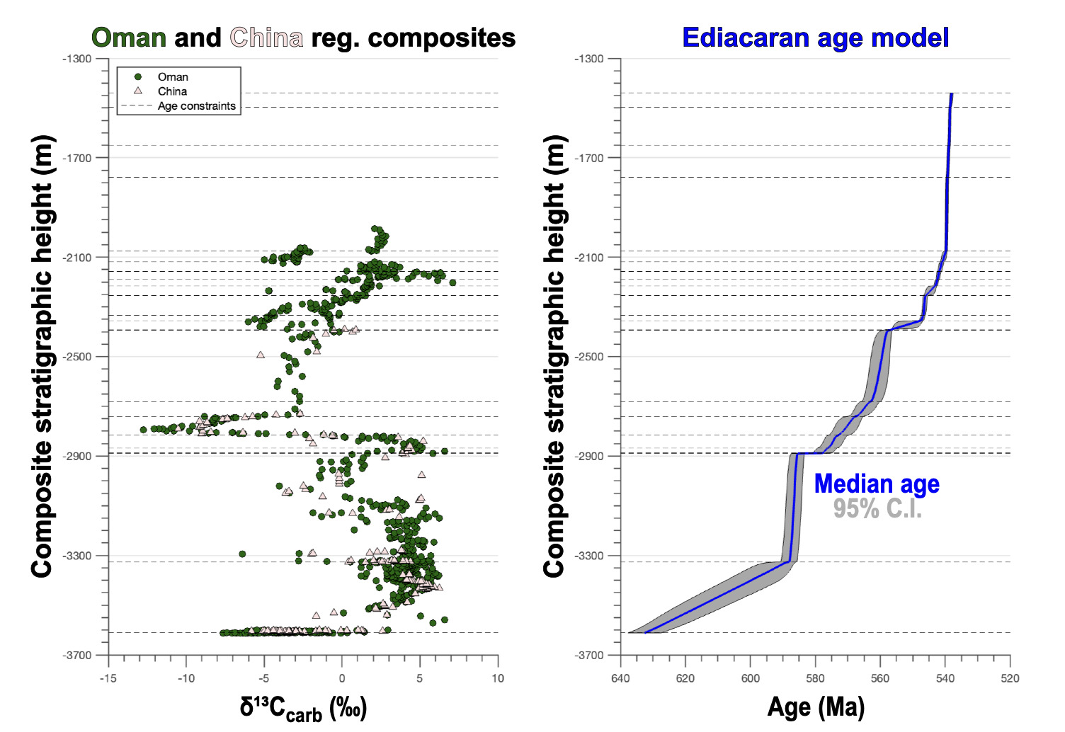
I select two Ediacaran regional composite stratigraphic records (from Oman and China; adopted from Hagen & Creveling, 2024) to demonstrate the proposed iterative approach with real data (Figures 4 and 5). These regional composite stratigraphic records were assembled using a dynamic time warping stratigraphic correlation algorithm called Align (Hagen et al., 2024; Hay et al., 2019) to position each constituent record (25 individual records make up the Oman regional composite record from Allen et al. (2004), Fike et al. (2006), Fike and Grotzinger (2008), Osburn et al. (2015), and Rooney et al. (2020), and 5 individual records make up the China regional composite record from Zhu et al. (2007), Zhu et al. (2013), and Yang et al. (2021)), as described in Hagen and Creveling (2024). Specifically, each record is a carbonate carbon isotope ($\boldsymbol{\delta}^{13} \mathbf{C}_{\text {carb }}$) time-series and Align varies geologically relevant penalty functions to best-fit time-series records (in a least-squares sense) to an identified target record. As such, every horizon in these regional composite records is more specifically a horizon with a paired $\boldsymbol{\delta}^{13} \mathbf{C}_{\text {carb }}$ value as collected, measured, and reported in those primary contributions (meaning that some carbonate horizons may not be represented by these regional composite records if they were not sampled for $\boldsymbol{\delta}^{13} \mathbf{C}_{\text {carb }}$ and all siliciclastic horizons are neglected; although note that the presence of these horizons can still be inferred due to portions of stratigraphic meterage lacking $\boldsymbol{\delta}^{13} \mathbf{C}_{\text {carb }}$ values). This algorithmic approach to stratigraphic correlation, and the iterative accumulation rate analysis presented herein, is not limited to $\boldsymbol{\delta}^{13} \mathbf{C}_{\text {carb }}$ records, as Align has been demonstrated to work well synchronizing paleomagnetic secular variation and ice firn density data as well (Hagen et al., 2020; Hagen & Harper, 2023), meaning that these analyses could be replicated using any kind of stratigraphic age-depth data. These Ediacaran regional $\boldsymbol{\delta}^{13} \mathbf{C}_{\text {carb }}$ composite records have accompanying high-resolution age-depth models derived through a Bayesian approach (Hagen & Creveling, 2024; Schoene et al., 2019; Trayler et al., 2019). For more details about the construction of these regional $\boldsymbol{\delta}^{13} \mathbf{C}_{\text {carb }}$ composite records and the Bayesian age-depth model, please refer to Hagen and Creveling (2024). While there are many horizons with paired $\boldsymbol{\delta}^{13} \mathbf{C}_{\text {carb }}$ values in each of these regional $\boldsymbol{\delta}^{13} \mathbf{C}_{\text {carb }}$ composite records, there is the potential for bias in the resulting accumulation rates towards carbonate rocks (the thicknesses of interbedded siliciclastic units are included in the composite meterage, but accumulation rates cannot be calculated for individual siliciclastic horizons). In theory, ages could be assigned to these siliciclastic horizons retroactively via interpolation, but that could introduce potential bias in our results and is beyond the scope of this contribution. Note that the resulting stratigraphic completeness estimates can only be as accurate as the age-depth models that they are based on. For example, linear age models may not capture the nuanced depositional history of a given record and may lead to inaccurate completeness estimates.

Figure 4.Ediacaran regional $\boldsymbol{\delta}^{13} \mathbf{C}_{\text {carb }}$ composite records for Oman and China with the corresponding Bayesian age model.

The Oman regional $\boldsymbol{\delta}^{13} \mathbf{C}_{\text {carb }}$ composite record (green) is composed of 25 individual $\boldsymbol{\delta}^{13} \mathbf{C}_{\text {carb }}$ records, and the China regional $\boldsymbol{\delta}^{13} \mathbf{C}_{\text {carb }}$ composite record (pink) is composed of 5 individual $\boldsymbol{\delta}^{13} \mathbf{C}_{\text {carb }}$ records, both of which were assembled using a dynamic time warping stratigraphic correlation technique (left; Hagen and Creveling, 2024). Dashed horizontal lines in each panel represent geochronologic age constraints incorporated into the Ediacaran Bayesian age model (median age shown in blue and the $95 \%$ confidence interval shown in grey; right). Both regional $\boldsymbol{\delta}^{13} \mathbf{C}_{\text {carb }}$ composite records and the corresponding high-resolution age model are adopted from Hagen and Creveling (2024). This plot is adapted from Hagen and Creveling (2024).

Figure 5.Sadler plots and completeness estimates for the Ediacaran Oman (above) and China (below) regional $\boldsymbol{\delta}^{13} \mathbf{C}_{\text {carb }}$ composite records.

Sadler plots (left) constructed using all of the accumulation rate and duration data calculated using the iterative approach (as in Figures 2 and 3; see Methodology). Some of the data from horizons with the oldest overlying ages (warmer colors) are obscured by data from younger horizons (colder colors). Completeness plots (right) indicate that these two regional composite records differ in their preservation (unlike the synthetic records in Figures 2 and 3), with the $50 \%$ completeness interval estimated at $\sim 11.9 \mathrm{Myr}$ in Oman versus $\sim 3.6 \mathrm{Myr}$ in China (1-Myr completeness estimates are $\sim 22 \%$ and $\sim 37 \%$, respectively). Horizontal red dashed lines indicate the stratigraphic completeness at an interval of 1 Myr. Vertical red dashed lines indicate the interval corresponding to $50 \%$ stratigraphic completeness.

UNDERSTANDING ACCUMULATION RATE TRENDS WITH SYNTHETIC RECORDS

Using the three synthetic age-depth models, I investigated how Sadler plots that contain every possible accumulation rate calculation for a stratigraphic record correspond to the age-depth models (see Figures 1 and 2). In the simplest example (record 1), there are two periods of steady accumulation separated by a geochronologic knickpoint (Figure 1). This knickpoint appears in the corresponding Sadler plot, where the lowermost row of data points (Figure 2A) represents the full suite of accumulation rate–durations for the uppermost horizon (see Figure 1A). The knickpoint in this lowermost row of data in the Sadler plot directly corresponds to the knickpoint in the age-depth model. As the Sadler plot is filled out through the addition of accumulation rate-duration suites from the other horizons, this knickpoint migrates left and up (see Figure 2A). This example provides intuition as to how a given accumulation rate–duration contour (from a suite of accumulation rate–duration data for an individual horizon) migrates through Sadler plots. Contour migration can also be clearly observed in synthetic record 3, with the lower right most arc of data (shown in green in Figure 2A) representing a single suite of accumulation rate–duration data from the logarithmic age model (Figures 1 and 2). As each accumulation rate–duration data suite is added to the plot, this contour migrates up and left (Figure 2A). The age-colored data points highlight how the horizon from which this data suite is calculated is moving up-section (becoming younger) as the contour moves. In the case of synthetic record 2, the resulting accumulation rate–duration contour is more complicated and irregular, reflecting the randomized horizon spacing (Figures 1 and 2). However, the same upward and leftward motion can be observed. The Sadler plot for synthetic record 2 compares most closely with those constructed from the Ediacaran regional $\boldsymbol{\delta}^{13} \mathbf{C}_{\text {carb }}$ composite records (although it is still very simplified due to its relatively short depositional history and simplified underlying assumptions in comparison).

In terms of stratigraphic completeness, the differences between these three synthetic age-depth models are relatively small (Figure 2). Across synthetic age-depth models 1–3 the estimated 1-Myr completeness was ~44%, ~50%, and ~63%, respectively (Figure 2). Furthermore, the 50% interval was 1.5 Myr, 1.0 Myr, and 0.3 Myr, respectively (Figure 2). These results demonstrate that although horizon thickness was randomized in synthetic age-depth model 2, the overall preservation was still very similar to synthetic age-depth model 1. Synthetic age-depth model 3 differs more substantially, which is not surprising when comparing the age-depth models themselves: for instance, it hosts more closely spaced horizons throughout much of the record (Figure 1).

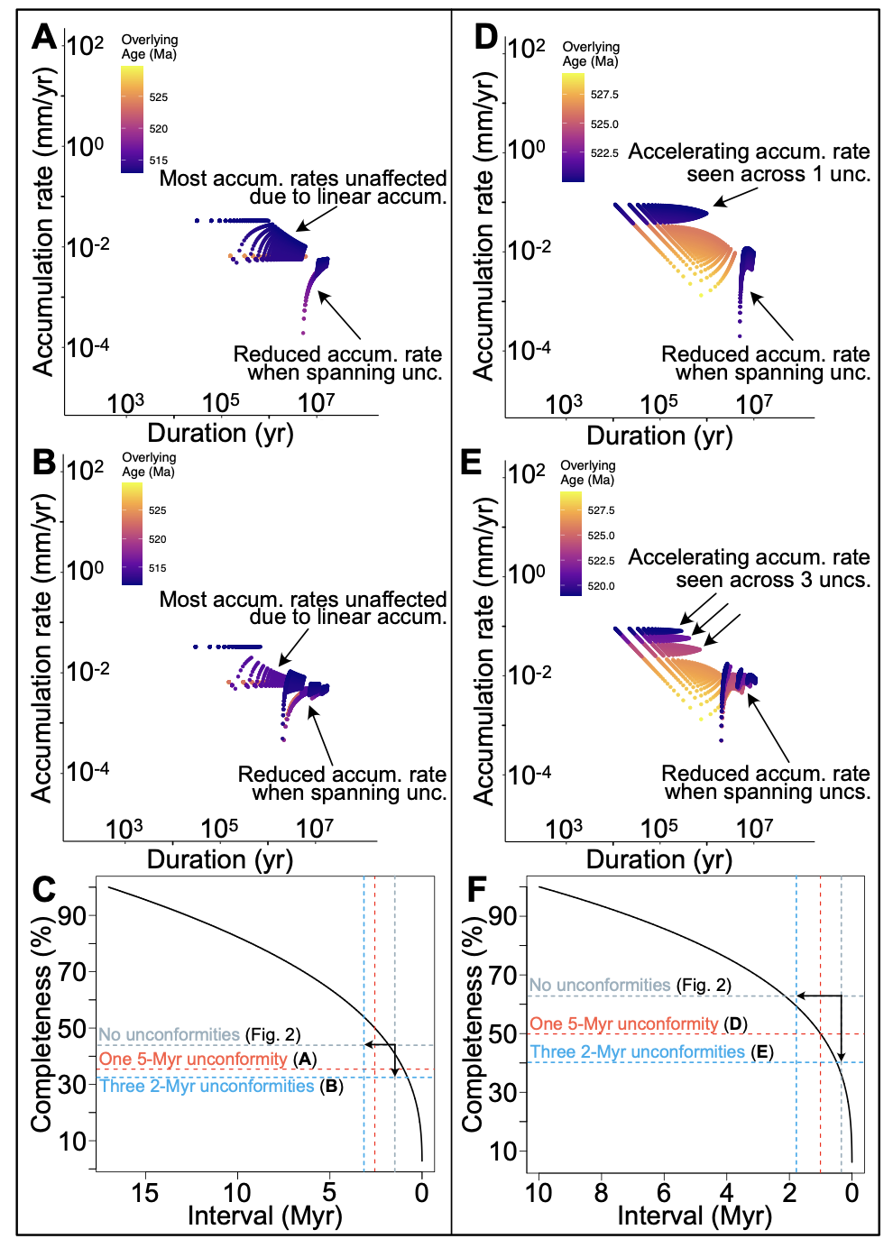
Adding unconformities to these synthetic records complicates their accumulation histories and the resulting Sadler plots (Figure 3). While the added unconformities do not substantially impact the Sadler plots for synthetic record 1 (Figure 3A–B), they have a more significant impact on synthetic record 3 (Figure 3D–E). Because accumulation rates are linear in synthetic record 1, accumulation rates are not changed by the unconformity unless the specific stratal pairing in question spans the unconformity (in which case the accumulation rate will be reduced; Figure 3A–B). In synthetic record 3, accumulation rates are accelerating through time, and this is clearly seen in the Sadler plot with each unconformity isolating accumulation rate–duration regimes (see different colored lobes in Figure 3D–E). As was the case with synthetic record 1, stratal pairings that span unconformities result in lower accumulation rates than they would otherwise (by necessity). In Figure 3C and F, the impact of these unconformities can be seen on the resulting completeness estimates, with greater missing time (more or longer unconformities) leading to lower completeness (as expected). While increasingly sophisticated synthetic age-depth models could be used to further explore how various depositional histories are reflected in Sadler plots, these three simple synthetics offer insight into interpreting more complex Sadler plots resulting from real age-depth models (Figures 4–6).

APPLICATION TO EDIACARAN REGIONAL $\boldsymbol{\delta}^{13} \mathbf{C}_{\text {carb }}$ COMPOSITE RECORDS

Short-term versus long-term accumulation rates

I calculate accumulation rates at two different resolutions— referred to as “short-term” and “long-term”—for the Ediacaran regional $\boldsymbol{\delta}^{13} \mathbf{C}_{\text {carb }}$ composite records (Figure 6). Short-term accumulation rates are simply the difference in height over the difference in age between two adjacent horizons. I refer to these rates as “short term” because they only reflect accumulation over a relatively short interval of time. In comparison, long-term accumulation rates result from the iterative process described above and are the mean of every accumulation rate calculated between every underlying horizon, j, and a given horizon, i:

$$\frac{\sum_{j = 1}^{n}s_{i,i - j}}{n}$$

This rate reflects accumulation between the base of the section and the horizon in question, representing a relatively long interval of time (hence the long-term nomenclature). Because of the relevant time scales, short-term accumulation rates are more likely to be influenced by faster, transient processes, while long-term rates should reflect slower, background processes.

Figure 6.Interpreting depositional history from high-resolution accumulation rates and Sadler plots.

Short- and long-term accumulation rates from China and Oman are compared (A) and demonstrate consistent trends in accumulation over time. For example, both the cap carbonate and Shuram carbon isotope excursions (CIEs) were characterized by relatively slow accumulation rates with respect to other Ediacaran intervals. In both records, accumulation rates increased prior to an interval lacking$\boldsymbol{\delta}^{13} \mathbf{C}_{\text {carb }}$ values that corresponds to the Gaskiers glaciation and the Oman Khufai–Shuram Formation unconformity (when $\boldsymbol{\delta}^{13} \mathbf{C}_{\text {carb }}$ values resume prior to the Shuram CIE, accumulation was suppressed, barely elevated above early Ediacaran background levels between ~620–600 Ma). In Oman, accumulation rates appear to have increased across the late Ediacaran, peaking near the Ediacaran–Cambrian boundary. These same trends can be observed with iterative Sadler plots (B), where each data point represents the mean accumulation rate and duration across the suite of values calculated for each overlying horizon through the iterative accumulation rate technique (the grey error bars depict the standard deviation of these accumulation rate and duration suites). These data are colored according to overlying horizon age, showing how the long-term accumulation–duration relationship varies across time for each record. For example, the carbon isotope gap coincident with the Gaskiers glaciation, as well as the Shuram CIE, can both be identified and are indicated in the plots. The increase in accumulation rate across the Ediacaran in Oman is also apparent, with younger samples progressively trending towards the upper left.

Iterative Sadler plots

I present a modified version of the classic Sadler plot (accumulation rate versus duration in log-log space), where long-term accumulation rates (see above) are plotted against long-term duration. I calculate long term duration in the same way as long-term accumulation rate:

$$\frac{\sum_{j = 1}^{n}d_{i,i - j}}{n}$$

I also plot uncertainties (±1 standard deviation) in long-term accumulation rate and duration. Finally, I color data according to overlying horizon age. This plot, hereafter referred to as an iterative Sadler plot (Figure 6), provides the stratigrapher a sense of the total variability in accumulation rate and duration (via the uncertainty bars) for the stratigraphic section (akin to classic Sadler plots; see Figure 5) while also containing information about the depositional history (via the age-colored long-term accumulation rate-duration data).

Ediacaran accumulation histories

The Sadler plots that result from the Ediacaran regional $\boldsymbol{\delta}^{13} \mathbf{C}_{\text {carb }}$ composite records are more complex than the synthetic age-depth models (Figures 2, 3 and 5) with multi-phase depositional histories. Some of these phases have clear accumulation rate–duration contours that migrate up and left like the contours observed in the synthetic age-depth models (e.g., see the purple and navy data in the Oman Sadler plot; Figure 5). The Sadler plots indicate that the earliest Ediacaran accumulation rates (warm colored data in Figure 5) cluster at slower rates than all other Ediacaran intervals. Ediacaran accumulation rates substantially increase between ~600–580 Ma in both regional $\boldsymbol{\delta}^{13} \mathbf{C}_{\text {carb }}$ composite records before falling again soon after ~580 Ma (Figure 5). In Oman, accumulation rates were again elevated from ~560–540 Ma (the China regional $\boldsymbol{\delta}^{13} \mathbf{C}_{\text {carb }}$ composite record does not capture deposition younger than ~560 Ma).

The Ediacaran completeness plots indicate that these two regional $\boldsymbol{\delta}^{13} \mathbf{C}_{\text {carb }}$ composite records differ substantially in their preservation (in comparison to the synthetic age-depth models in Figure 2). The Ediacaran Oman and China 50% interval estimates were ~11.9 Myr and ~3.6 Myr, respectively, with corresponding 1-Myr completeness estimates of ~22% and ~37% (Figure 5). These 50% interval estimates indicate that one out of every two ~11.9 Myr or ~3.6 Myr intervals of time are represented by at least some rock in the Ediacaran Oman and China stratigraphic records. Conversely, the 1-Myr completeness estimates indicate that roughly one out of every four and one out of every three 1-Myr intervals of time are represented by at least some rock in the Ediacaran Oman and China stratigraphic records. These completeness estimates are markedly worse than those from the synthetic age-depth models, which is not surprising as the synthetic age-depth models are unusually high-resolution (100 horizons spread over 100 m across 12 Myr, with horizon thickness varying between the synthetic age-depth models) when compared with the real Ediacaran age-depth models.

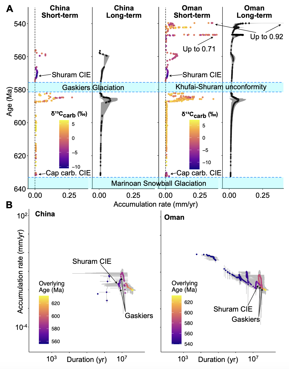
I calculated short-term and long-term accumulation rates for both the China and Oman Ediacaran regional $\boldsymbol{\delta}^{13} \mathbf{C}_{\text {carb }}$ composite records (Figure 6A). Comparing the short- and long-term accumulation rates, the long-term rates are sympathetic albeit more muted (short- and long-term accumulation rates shift simultaneously but long-term rates are of smaller magnitude; Figure 6A). For example, both short- and long-term accumulation rates spike in Oman and China between ~590–580 Ma. The accumulation rate trends between Oman and China are quite similar, which is not surprising since the age-depth model used for these calculations resulted from the alignment of these (and other) regional $\boldsymbol{\delta}^{13} \mathbf{C}_{\text {carb }}$ composite records (see Hagen & Creveling, 2024). In Oman, accumulation rates (both short- and long-term) increase across the Ediacaran, peaking near the Ediacaran–Cambrian boundary at ca. 540 Ma (Bowring et al., 2007). There are two additional Ediacaran accumulation rate spikes: one at ~560 Ma in Oman and China; and another at ~547 Ma in Oman (note that the China regional $\boldsymbol{\delta}^{13} \mathbf{C}_{\text {carb }}$ composite does not record deposition younger than ~560 Ma).

One interesting observation from these data is that accumulation rates (both short- and long-term) are relatively slow (< 0.1 mm/yr; Figure 6) during the two prominent carbon isotope excursions reported from the Ediacaran Period: the cap carbonate excursion in the earliest Ediacaran immediately following the Marinoan Snowball Earth glaciation; and the Shuram excursion in the middle Ediacaran, which occurs ~6 Myr after the Gaskiers glaciation (Hagen & Creveling, 2024; Rooney et al., 2020). The Gaskiers glaciation, the geographic extent of which is contentious, occurred between 580.90 ± 0.40 Ma and 579.88 ± 0.44 Ma (Pu et al., 2016), which is situated in the Hagen and Creveling (2024) Ediacaran age-depth model during an interval lacking $\boldsymbol{\delta}^{13} \mathbf{C}_{\text {carb }}$ values and corresponding to the prominent Khufai–Shuram Formation unconformity reported in Oman (e.g., Fike et al., 2006). While it is unclear whether these glaciations are related to the carbon isotope excursions, perhaps the glaciations played a role in suppressing accumulation rates during those intervals. This finding is in agreement with previous accumulation rate estimates for the Marinoan Glaciation, which differentiated Snowball glaciations from those in the Phanerozoic Eon due to relatively slow (but comparable to those reported herein) Snowball glaciation accumulation rates (Partin & Sadler, 2016).

We can observe these same events and interpret the depositional histories of these stratigraphic records using iterative Sadler plots (Figure 6B). For example, the depositional gap in these records coincident with the Gaskiers glaciation is shown as an age gap in the mean long-term accumulation rate–duration data in both China and Oman. Furthermore, the small uptick at the time of the Shuram excursion can also be seen. The overall increase in accumulation rate across the Ediacaran is clear in Oman, with younger data trending up and left. The power of this visualization is that stratigraphers get a glimpse of variability in accumulation rate over time (grey uncertainty bars) while also depicting the depositional history (age-colored mean long-term accumulation rate–duration data).

The Sadler Effect is still evident in these, and all other Sadler plots, demonstrating decreased accumulation rate with increased duration. When comparing these calculated short- and long-term accumulation rates with a global compilation of shallow marine carbonate accumulation rates (where carbonate accumulation rates range from ~10^-5–10³ mm/yr; Kemp & Sadler, 2014), these rates appear to be reasonable. Due to the fractal characteristics of sediment accumulation, the completeness of a given stratigraphic record depends on the completeness interval in question (Sadler, 1999). If one sought to ensure at least 50% stratigraphic completeness when working with these Ediacaran records, relatively long intervals would need to be considered. In the Oman and China basins, the 50% interval is ~11.9 Myr and ~3.6 Myr, meaning that most of the rock record is typically missing if assessed at a higher resolution than ~11.9 Myr and ~3.6 Myr, respectively. This finding severely limits the stratigraphic questions that can be confidently assessed at a 1-Myr resolution and finer, and even suggests that assessments at a 10-Myr resolution may be questionable in some Ediacaran basins, such as Oman. These accumulation rate analyses, afforded by a high-resolution age-depth model, offer new insight into the depositional histories of these Ediacaran basins, namely that the post-Marinoan and Shuram carbon isotope excursions were characterized by relatively slow accumulation rates and that these Ediacaran basins have relatively low completeness at the 1-Myr interval (22–37%). These same assessments should be made for other Ediacaran basins to assess if this level of completeness is typical for this interval of Earth history, and to further elucidate relationships between Ediacaran carbon isotope excursions, accumulation rates, and glaciations.

NEW QUANTITATIVE TOOLS FOR THE STRATIGRAPHY COMMUNITY

The analyses presented herein prove a powerful tool for interpreting depositional histories of individual stratigraphic records. As stratigraphic research is becoming more data-dense, the need for quantitative tools that aid in interpreting these datasets is also growing. To facilitate this shift, I provide a function, written in the free and open-source R language, that replicates the analyses presented herein for any stratigraphic record with an accompanying age-depth model. As the community moves towards more advanced quantitative approaches, such as accumulation analyses (this work), correlation algorithms (e.g., Hagen et al., 2024; Sylvester, 2023), chronology tools (e.g., Johnstone et al., 2019; Meyers, 2014), image analyses (e.g., Howes et al., 2021; Mehra & Maloof, 2018; Reilly et al., 2017), geochemical modeling tools (e.g., Ahm et al., 2021; Hagen, 2024; Trower et al., 2024), and stratigraphic modeling tools (e.g., Borgomano et al., 2020; Busson et al., 2019; King & Creveling, 2022), special efforts should be made to develop open-source, easy to use, and archived packages to ensure that these community tools can be widely used by all.

CONCLUSIONS

In this contribution, I explore quantitative and reproducible techniques for analyzing sediment accumulation rates derived from stratigraphic records with high resolution age-depth models. As expected, the same negative power law relationship between sediment accumulation rate and duration originally documented by Sadler (1981) characterizes individual stratigraphic records. Much can be gleaned from leveraging Sadler plots to understand the depositional history of individual stratigraphic records that have accompanying high resolution age-depth models. For example, iterative Sadler plots, a variant on the classic plot presented herein, can offer a glimpse at both the depositional history of an individual record and the specific negative power law relationship between accumulation rate and duration. When assessing two Ediacaran regional $\boldsymbol{\delta}^{13} \mathbf{C}_{\text {carb }}$ composite records, I find that accumulation rates were generally low during the early Ediacaran with a marked increase between ~600–580 Ma and a pronounced peak near the Ediacaran–Cambrian boundary. Two large, documented carbon isotope excursions during the Ediacaran (the cap carbonate excursion and the Shuram excursion) are characterized by relatively slow accumulation rates following glaciations (the Marinoan and Gaskiers glaciations, respectively). Completeness estimates for these regional $\boldsymbol{\delta}^{13} \mathbf{C}_{\text {carb }}$ composite records were ~22% and ~37% at a 1-Myr interval (for Oman and China, respectively; 50% completeness intervals were estimated at ~11.9 Myr and ~3.6 Myr, respectively). This analytical approach for understanding local accumulation histories will allow for a more nuanced understanding of these records, for example, facilitating the assessment of episodic and periodic accumulation (Sadler, 1994). Lastly, I provide a free and open-source function that can reproduce these analyses for any stratigraphic record with an accompanying age-depth model.

ACKNOWLEDGEMENTS

I acknowledge support from the NSF Graduate Research Fellowship Program, the ARCS Foundation Fellowship, and the Agouron Geobiology Postdoctoral Research Fellowship. P. Sadler, A. Meigs, R. Mahon, and K. Jay provided helpful conversations. I thank J. Creveling, E. Trower, A. Mehra, J. Harper, and B. Reilly for their careful reviews of earlier drafts and for providing invaluable support. I also thank reviewers Steven Holland and Peter Sadler for their constructive and encouraging feedback that greatly improved this contribution, as well as Daan Beelen for editorial handling.

Open Science

All coding and analyses for this contribution were conducted in the free and open-source R language (R Core Team, 2022). To facilitate quantitative analysis across the stratigraphy community, an R function is provided that performs the necessary iterative calculations and generates the plots discussed herein for any stratigraphic record with an accompanying age-depth model (see Discussion). The function is available at https://github.com/CedricHagen/Iterative-Sadler-Plots.