

INTRODUCTION
Much effort within the discipline of stratigraphy has been expended on addressing the inverse problem. Given a stratigraphic succession of beds displaying varying sedimentologic characteristics, stratigraphers seek to reconstruct the geomorphic processes and boundary conditions responsible for generating them. We can conceptualize strata, then, as the “output” of geomorphic process “inputs” linked with autogenic, tectonic, climatic, and eustatic conditions. The foundational geologic principles of Uniformitarianism and Walther’s Law rely on the fidelity of the relationship between geomorphic inputs and stratigraphic outputs. And the extensive development, testing, and application of lithofacies models over numerous decades confirms the robustness of this geomorphology–stratigraphy correspondence (e.g., James & Dalrymple, 2010; Reineck & Singh, 1980). However, also well documented are the ways in which stratigraphy fails to accurately capture geomorphic evolution.
Sadler (1981) documented a systematic decrease in sedimentation rates as the time interval over which they are estimated increases. Several researchers have shown that the stratigraphic record is temporally incomplete (i.e., only a proportion of geologic time is represented by strata), and that the severity of incompleteness increases as the timescale of interest approaches the rate of many geomorphic processes (e.g., channel avulsion, fluvial bar accretion, dune migration) (Dott, 1983; Hajek & Straub, 2017; Sadler, 1981; Straub et al., 2020). Some estimates of incompleteness imply that, on the bed-scale, only around one millionth of the total time a system is active can be expected to be represented as strata (Holbrook & Miall, 2000; Miall, 2015; Paola et al., 2018). Such undersampling raises concerns that the preserved strata may be unrepresentative of the geomorphic processes that constructed them. Unconformities of varying duration are the underlying cause behind this incompleteness, but recent work further suggests that the mechanism generating unconformities (i.e., stasis versus erosion) also varies with the timescale under consideration (Straub & Foreman, 2018). Furthermore, there is good reason to suspect that the beds ultimately preserved as strata may exhibit different statistical properties (e.g., thin-tailed, exponential distributions) than the geomorphic surface elevation variations (e.g., heavy-tailed deposition and erosional events) that generated them (Straub et al., 2012). Yet these issues may be less severe than originally thought, with recent work suggesting that the stratigraphic record is not biased towards rare, extreme events, but captures the ordinary geomorphic events of a transport system (Paola et al., 2018). This is likely facilitated by the nesting of small-scale (e.g., ripples) geomorphic process products within larger (e.g., bar migration) geomorphic process products (Ganti et al., 2020).
This study addresses the stratigraphic inverse problem by applying machine learning (ML) approaches to an experimental fluviodeltaic basin dataset (TDB17-1; Fig. 1A; Straub et al., 2023). Stratigraphic experiments, wherein sediment and water are fed into a basin with prescribed base level constraints, capture many of the behaviors and phenomena of field-scale sediment transport systems (Paola et al., 2009). They have provided significant insight into how geomorphic processes are recorded within stratigraphy, oftentimes in nonintuitive ways (Paola et al., 2009; Sylvester et al., 2024). Importantly, the experiments allow the precise tracking of geomorphic processes to the preserved strata and they can be incredibly data-rich. ML approaches can identify complex patterns in large datasets that may not be apparent through traditional analytical methods. Herein, we leveraged large-n data (greater than 14 million points) of experimental geomorphic processes, linked directly with their stratigraphic deposits, to train ML models whose success could then be assessed with similarly large-n data left out of the ML training procedure (i.e., the validation data set). This approach allows us to evaluate how well computational methods can predict lost depositional information from preserved stratigraphic characteristics. Specifically, we are interested in reconstructing the attributes of vacuities (i.e., the representation of time and deposition removed by erosion; Wheeler, 1964) that create incompleteness within stratigraphy.
METHODOLOGY
Experimental Basin
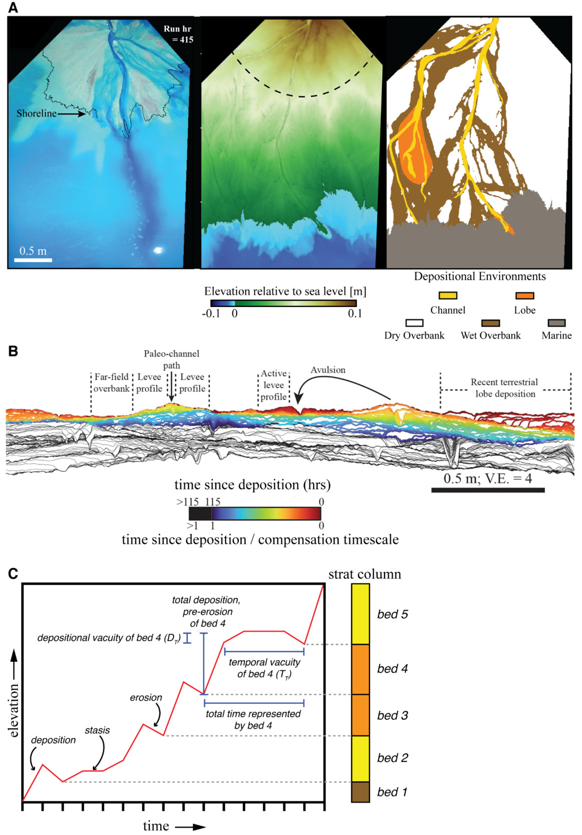
Full details of the TDB17-1 experimental setup can be found in Straub et al. (2023), and are summarized herein. The experiment (TDB17-1) occurred in a 4.2 m × 2.8 m × 0.65 m basin housed at Tulane University’s Sediment Dynamics Laboratory. A point source of sediment flux and water discharge were held constant at 3.9 × 10⁻⁴ kg/s and 1.7 × 10⁻⁴ m³/s, respectively, as the basin evolved (Fig. 1A). Base level was set to steadily rise at 0.1 mm/hr via a computer-controlled weir with sub-millimeter precision. The sediment mixture was modeled after Hoyal and Sheets (2009), with particle sizes ranging from approximately 1–1000 μm (median 67 μm). Small amounts of bentonite, cat litter, and granular polymer were added to increase cohesion, enabling relatively narrow and deep channels to form from subcritical flows transporting fine-grained sediment in suspension and coarse-grained sediment as bedload. To visualize stratigraphic architecture, a quarter of the coarsest 23.5% of the sediment distribution was dyed red, with the remainder consisting of white particles. With experimental boundary condition inputs held constant (i.e., sediment flux, water discharge, base level rise rate) and the system, on net, purely aggradational, the geomorphic evolution and stratigraphy generated in TDB17-1 can be considered autogenic (Straub et al., 2023). A FARO Focus3D-S 120 laser scanner collected topographic point clouds twice per run-hour over the 560-hour aggradation stage of the experiment. The scanner also collected digital images, such that every topographic point was co-registered with RGB color. One of these two point cloud maps occurred with flow on and water dyed blue to aid in identification of geomorphic environments (e.g., wet vs. dry overbank, active vs. inactive channels). The experimental run time, aggradation rate, and self-organized channel depths (~10 mm), facilitated the construction of many channel depths worth of strata (Fig. 1B). Paused scans at the end of each run-hour provided high-precision topography, converted to digital elevation models with 5 mm grid spacing horizontally and < 1 mm vertical resolution (Fig. 1B). This temporal and spatial resolution captures mesoscale dynamics including channel migration and avulsion events, and provides precise time series of erosion, deposition, and geomorphic stasis events along with maps of depositional environment classifications (Fig. 1A&C). Straub et al. (2023) mapped depositional environments by hand. Linear flow features with sharp blue intensity (dyed water) defined channels, with levee crests separating them from overbank environments. Lobes were mapped where channels lost confinement, typically before reaching base level, and were largely composed of coarser sand fractions. Areas of the experimental surface not a channel nor a lobe and inundated with flow were classified as wet overbank, those areas without inundation were classified as dry overbank. This yields a data set of 232,686,720 elevation measurements across the entire experimental surface over the 560-hour experiment and a corresponding depositional environment. From this data the magnitude and duration of geomorphic depositional, erosional, and stasis events behind each stratigraphic bed can be determined and be precisely linked to a subenvironment category (i.e., channel, lobe, dry floodplain, wet floodplain, marine).
_overhead_.png)
A three-dimensional (3D) tensor of data was obtained from the TDB-17-1 experiment for this study (data available at Tulane Sediment Dynamics and Quantitative Stratigrpahy Group’s collection at https://sead2.ncsa.illinois.edu/collection/596d28c5e4b05e3417b2096f). The x- and y- horizontal coordinates capture a grid of the experimental surface, and the vertical z-axis represents time steps of overall runtime. Each cell represents the elevation of that location at timestep n. Starting from time zero at each location, we tracked changes in elevation over timesteps to build discrete beds or, more generally, “layer objects” that are defined as the accumulated sediment thickness between two, successive, preserved surfaces of erosion. This is the same definition of a bed as used in Straub et al. (2012).
Thus, for each layer object in the experiment the following attributes are known and used in our machine learning models: (1) the total accumulated, pre-erosional depositional thickness of a bed; (2) the vertical amount of erosion a bed experienced prior to preservation (i.e., the depositional vacuity, DT); (3) the preserved bed thickness; (4) the total time represented by a bed (i.e., the sum of the duration a bed was in deposition, stasis, and erosion); (5) the time represented by strata removed by erosion (i.e., the temporal vacuity, TT); (6) the preserved bed duration calculated from the long-term linear sedimentation rate of the stratigraphic column at the end of the experiment (i.e., the preserved bed thickness divided by long-term sedimentation rate of the entire stratigraphic column); and (7) the environment the bed was deposited in, either channel, lobe, dry floodplain, or wet floodplain. Strata deposited in the marine environment were excluded from the models. In some cases, multiple environments contributed to a bed and we assigned it the environment that was most common in the resulting bed thickness. We also included an additional attribute, (8) a “high-erosion” tag that was assigned to a layer when the difference between the preserved bed thickness and pre-erosional depositional thickness exceeded 6.5 mm (the experiment’s average channel depth). Our ML models aim to predict attributes (2) DT and (5) TT, based on predictor attributes (3), (6), (7), and (8). Neither DT nor TT are directly observable in the field but directly pertain to stratigraphic completeness.
In alluvial and deltaic systems there is growing evidence that morphodynamic processes are strongly linked to channel flow depths (Straub et al., 2020). This appears to be the case for both experimental and field systems (Cardenas et al., 2023; J. Martin et al., 2018; Mohrig et al., 2000; Sheets et al., 2002; Straub et al., 2020), making flow depth a natural length-scale by which to non-dimensionalize the vertical spatial domain. Furthermore, several studies have identified a characteristic timescale, termed the compensation timescale (Sheets et al., 2002; Straub et al., 2020), that captures the typical time it takes for a stratigraphic layer to subside below the vertical zone of active geomorphic reworking and permanently enter the stratigraphic record (Fig. 1B; Straub et al., 2020). This compensation timescale is related to the topographic roughness of a geomorphic system and the long-term subsidence rate of a basin (Sheets et al., 2002; Straub et al., 2009). It offers a natural timescale that can be used to non-dimensionalize the time domain in experimental and field transport systems (Hajek & Straub, 2017; Straub et al., 2020). In the case of experiment TDB17-1, the average channel flow depth is ~6.5 mm and the compensation timescale is ~115 hours (Straub et al., 2023), and we evaluate the success of ML approaches scaled to these values. This non-dimensionalization allows us to more easily translate and illustrate the implications for field-scale systems.
Machine Learning
With the data structure established to represent key stratigraphic processes, a broad range of ML model families were evaluated to identify well-performing regression approaches, with subsequent refinement through hyperparameter optimization. Baselined models included simple linear regression, support vector machines, neural networks, and decision tree-based approaches. From initial baselines, neural networks and decision trees showed promise in learning the data’s patterns and inner representations. As both model families performed similarly, and given the lighter-weight approach of random forests, a random forest (RF) model was chosen to move forward, along with variants of that model. An RF model approach is an ensemble learning technique that trains multiple decision trees and combines their predictions through a weighting system to produce the final output. This ensemble technique allows RF models to excel at reducing overfitting and capturing non-linear relationships between input attributes and target attributes—important capabilities for stratigraphic reconstruction where depositional and erosional processes interact in complex ways. RF models have seen success in alternate applications in geological fields, such as lithology and facies prediction in cored wells (T. Martin et al., 2021) and classification of stratified geology (Silversides & Melkumyan, 2022).
With an RF approach selected, we fine-tuned the model by iteratively adjusting key parameters to achieve optimal performance. Key parameters included the number of trees in the ensemble, maximum tree depth, feature splitting criteria, and the minimum number of samples required for splitting or forming leaf nodes. Additional ensemble variants, including XGBoost (Chen & Guestrin, 2016) and AdaBoost (Freund & Schapire, 1997), were also tested. This process involved running multiple training iterations to identify the combination of parameters that yielded optimal performance for both depositional vacuity (DP)and temporal vacuity (TP) predictions. Model performance was evaluated using Mean Absolute Error (MAE) to measure prediction accuracy of a subset of data left out of the model and R² to measure a model’s contribution to variance in resulting predictions. Training data consisted of 500,000 data points, with a validation set including 100,000 data points, both sampled at random from a pool of ~14 million available data points. All data processing and ML model code available at https://doi.org/10.5281/zenodo.19464570.
RESULTS
Table 1 presents model performance metrics (MAE and R²) for all targeted attributes (i.e., depositional vacuity, DT, and temporal vacuity, TT) to predict, comparing cases with and without the high-erosion tag. Without the high-erosion tag, the RF model achieved a non-dimensionalized MAE of 0.3182 for predicting the depositional vacuity due to erosion (DP) and 0.0989 for predicting the temporal vacuity due to erosion (TP). When the high-erosion tag was included, performance improved substantially: non-dimensionalized MAE decreased to 0.1810 for DP and 0.0566 for TP. R² values reflect similar gains, where the DP R² increased from 0.4328 to 0.8150 with the addition of the erosional tag, and the TP increased from 0.0602 to 0.6859.
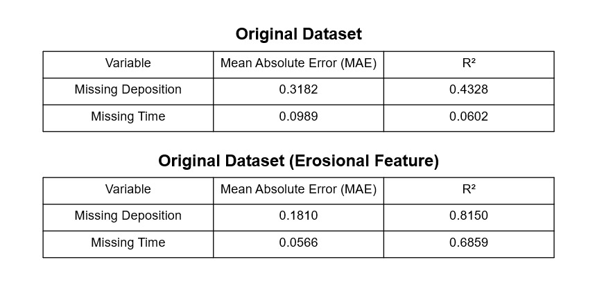
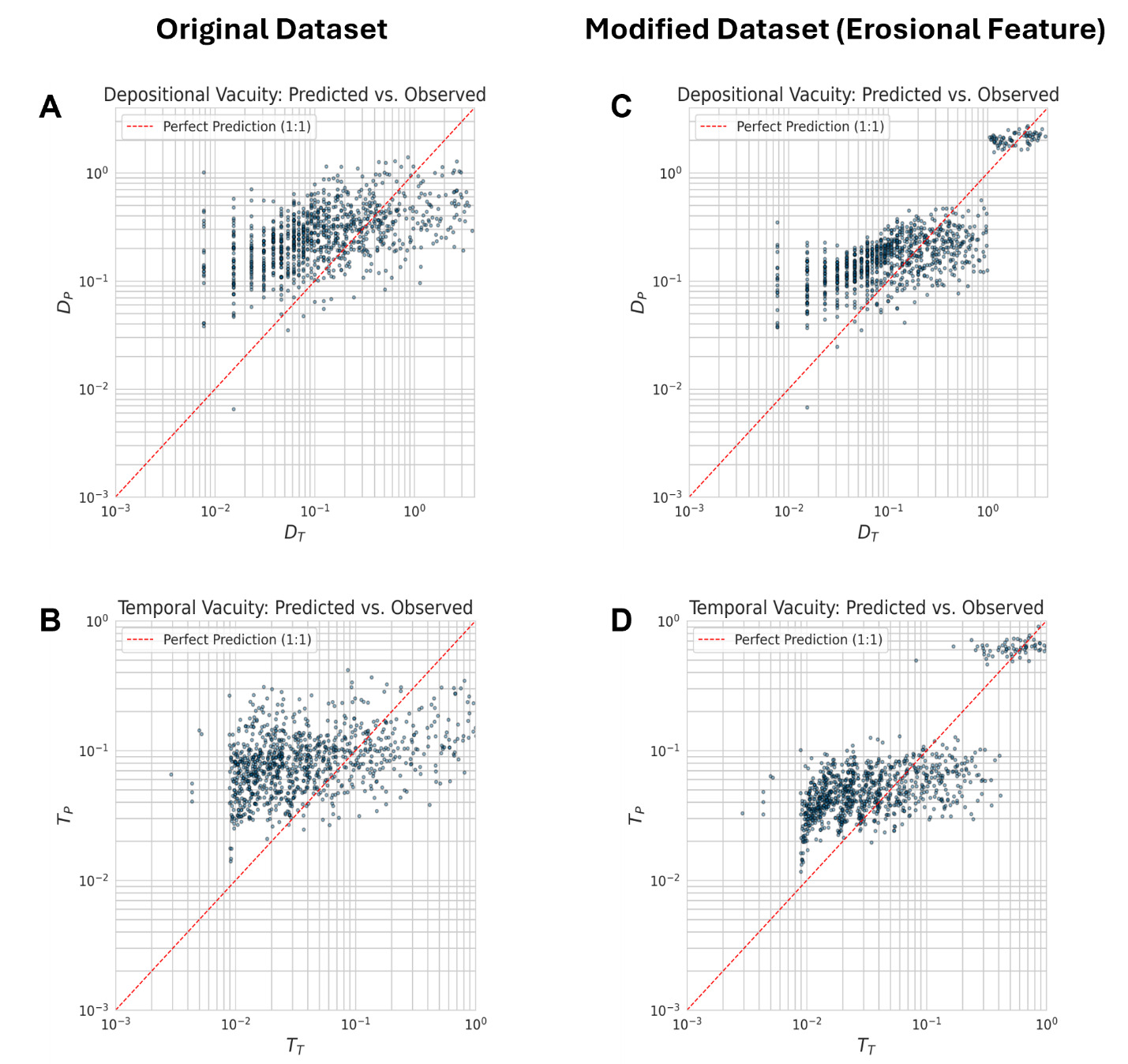
Figure 2A presents the relationship between predicted depositional vacuity DP and their a priori known vacuity (DT) for individual data points in the validation data set (i.e., data left out the model training) for models that did not or did include the high-erosional tag. Figure 2B presents the same relationship for the predicted temporal vacuity TP and known temporal vacuity due to erosion, TT. When the erosional tag is excluded, both predictions scatter broadly around the 1:1 reference line, reflecting weaker prediction power (Fig. 2A&B). And both notably struggle to recover larger amounts of deposition (DT > ~1.0) and longer durations of time (TT > ~0.4). With the tag included, points cluster more tightly around the 1:1 prediction line and overall dispersion decreases. Importantly, the inclusion of this high-erosion tag shifts predictions of larger DP and longer TP closer to the 1:1 line (Fig. 2C&D) as well as reducing the overpredictions that occur in small DP and short TP (Fig. 2C).
DISCUSSION
The underlying purpose of this study is to assess the effectiveness of machine learning (ML) techniques in recovering fundamental geomorphic information from incomplete stratigraphy. Building on previous ML applications in geologic phenomena reproduction, we leveraged the constructed controlling systems captured in experimental data, while critically, the high-precision measurements of temporal changes in these systems. This approach establishes defined model inputs while facilitating the transition to field applications where stratigraphic records are incomplete. Our reported model performance not only shows considerable accuracy of our models in reproducing the desired vacuities, but the importance of additional features being key contributors to underlying patterns. While these additional features are readily derived from high-precision temporal data in experimental settings, their identification and measurement in field settings proves difficult for many environments. Vacuities would be a quintessential example, by definition they represent strata once deposited then eroded and time once preserved as sediment, now gone. With our approaches to a high erosional tag (akin to a rapid channel incision event and a scour surface as a stratigraphic product), we defined methods to measure this feature in both our experimental data and within a field setting, while relying on differing key features of the measured environment. This approach can be further leveraged to produce comparable features for alternative experimental settings and field applications. As this addition of input features is a standard practice of ML optimization and performance, experimental data setups prove both effective in doing so, while possibly creating dependencies that are nonreproducible in a field setting.
Machine learning models can be improved in a number of ways. For example, larger training data sets, additional predictor attributes, and greater accuracy and precision of the pertinent measurements of all the attributes. However, to assess the generality of these ML models, a logical next step is to apply them across stratigraphic experiments run under different baseline conditions. Our RF model successfully recovers vacuity information from a cohesive fluviodeltaic system with single thread channels that evolved under autogenic conditions. But, can these same models be applied to noncohesive deltaic systems with multi-thread braided channels? To what extent do differences in grain size and proportions impact the mean absolute errors of the predictions? Moreover, how do base level fluctuations impact ML vacuity predictions? Intuitively, prediction quality will be reduced when using a model trained on one experiment but applied to another experiment (i.e., to what extent are models transferable?). The key issue to address is the extent to which each experimental system is unique and necessitates its own ML model. This has implications for application to field-scale basins which are more complex than experiments. It may be the case that ML models will need to be trained on several experimental data sets to produce something useful for field scale and/or certain domains of models can only be used in certain circumstances.
An additional challenge in experiment-to-field translation is ensuring real-world measurability of the attributes used in the predictions. Experiments are not just small-scale versions of field-scale geomorphic systems (Paola et al., 2009). For example, it is very difficult to match the fluid dynamic properties, such as the Froude and Reynolds numbers, of experiments to field-scale deltas (Paola et al., 2009). While both experiments and field deltas exhibit river bar formation and mouth bar deposition (scale-independent phenomena) experiments do not produce channels with ripples and dunes (scale-dependent phenomena). For these and future models researchers will want to find analogous features that are scale-independent (or testable scale-independent phenomena). The high-erosion tag models offer one example of this. In the experiment high-erosion is defined by the removal of at least one flow depth worth of elevation from the stratigraphic column. This is a binary, categorical predictor attribute. A plausibly equivalent attribute in a field setting could be a deep channel scour or significant relief on a disconformity surface into underlying strata in excess of a channel flow depth, which would be independently determined from bar clinoform relief. While the depth of erosion would only be an estimate, it would be sufficient to assign the binary categorical attribute. In our ML models even the addition of this one attribute substantially improves the quality of predictions. Other categorical attributes that could be used in future studies include clear evidence of stasis, either in the form of significant paleosol development (Kraus, 1999) or delicate, substrate surfaces preserved on bedding planes (e.g., surficial trace fossils, ripples) (e.g., Davies & Shillito, 2018). A categorical tag of clear stasis could then be included. Another possible avenue is incorporating a semi-quantitative scale such as a bioturbation index (e.g., Droser & Bottjer, 1986), commonly applied to marine strata, or a soil morphology index (e.g., Adams et al., 2011) to capture relative durations of stasis on stratigraphic surfaces. This semi-quantitative scale would not necessarily need a direct one-to-one mapping with experimental systems, but rather capture the phenomenon of a spectrum of stasis durations.
Our results are scaled by characteristic geomorphic phenomena that control both experimental and field systems (Sheets et al., 2002; Straub et al., 2009; Hajek et al., 2010; Straub et al., 2020; Wang et al., 2024). As such, our mean absolute errors of ~18% and ~6% for lost strata and lost time, respectively, from the high-erosion tag models can be tentatively translated into field-scales. Using realistic flow depths of 1-10 m for alluvial rivers, the implied mean absolute error would be ±0.18 m to ±1.8 m for predicting the amount of removed sediment from any given bed (sensu Straub et al., 2012) in a fluvio-deltaic setting. However, this estimate assumes the pertinent topographic roughness scale driving morphodynamics is a channel flow depth; some field systems exhibit roughness scales at several multiples of channel flow depths (e.g., Hajek et al. 2010; Wang et al., 2024). This implies our model may only recover missing strata on the scale of several meters. In terms of temporal vacuity, field-based estimates of compensation timescales are still comparatively rare, but appear to fall within 104 to 105 years (Hajek et al. 2010; Hofman et al., 2011; Li et al., 2016; Wang et al., 2024). If our ML approaches are transferable, it implies that time lost to vacuities could be reallocated to beds with errors of ~600 to ~6000 years. Additional work needs to occur in order to systematically apply experiment-based ML models to field-scales, but our results emphasize the potential of these models for addressing the pervasive incompleteness of the stratigraphic record. Specifically, they can reliably recover information lost to vacuities which produce paraconformities. In deeper geologic time these paraconformities have resisted quantitative efforts at extracting their time and stratal losses. Even minor constraints on the offset between the spatial and temporal domain in a stratigraphic column should aid in producing more accurate and realistic rates of paleobiologic and paleoclimatic change from proxy records recorded the stratigraphic record (Foreman & Straub, 2017; Straub & Foreman, 2018).
ACKNOWLEDGEMENTS
This research was supported by funding from internal Western Washington University grants (to R.B) and NSF grant EAR-1424312 (to K.M.S.)