
_based_on_maximum_flooding_surfaces_(mf.tiff)


**_xrf_cross_plots_comparing_calcium_(ca)_to_silicon_(si)__and_sulfur_(s)_to_iron_(fe).tiff)
INTRODUCTION
Well-log analysis, formation evaluation, and subsurface property modeling are an integral part of subsurface characterization for oil and gas exploration, carbon sequestration, geothermal development, mineral exploration, and water-resource characterization (Maries et al., 2017; Stumm & Como, 2017; Wallis et al., 2009; Williams & Lane, 1998). These workflows are typically performed on proprietary datasets using closed-source commercial software (e.g., Eriavbe & Okene, 2019). However, machine learning (ML) models and open-source datasets have led to major advances in the geosciences (Dramsch, 2020) due to their ease of use in high-level programming languages (e.g., Python) that have thorough documentation and community support. Developing reproducible workflows (e.g., reservoir property prediction) using open-source ML tools will allow researchers to investigate relationships and predictive performance on their own datasets. However, the large number of choices of ML models and methodologies (e.g., classification, regression) makes it difficult to select a particular model that will be effective for a specific use case (Raschka, 2018).
This study compares five open-source ML regression models for subsurface formation property prediction, utilizing well-log data and derived core-image statistics. We chose a regression methodology (predicting a value) instead of classification (predicting a label) because (1) numerous studies have explored classification (Bormann et al., 2020; Hall & Hall, 2017) and (2) regression tends to be a better choice for predicting continuous reservoir property values. We demonstrate this workflow using an open-source dataset focusing on the Dad Sandstone Member within the Lewis Shale in south central Wyoming, which is analogous to many submarine channel-fan deposits that host significant oil and gas reserves (Pyles & Slatt, 2007). While these data and models are from a specific sedimentary depositional environment, the findings and workflows are transferable to other environments (e.g., fluvio-deltaic systems, carbonate platforms) and datasets (e.g., borehole image-log, hyperspectral core images) as long as there are trusted training and testing datasets from those environments.
GEOLOGIC SETTING
This study examines Upper Cretaceous submarine fan deposits within the Greater Green River Basin (GGRB) in south central Wyoming (Fig. 1). The GGRB is an active hydrocarbon-producing basin with exploration activity dating back to the early 1950’s (Hettinger & Roberts, 2005). The cores in this study were retrieved from legacy vertical wells in several producing gas fields (Fig. 1; Asquith, 1975; Hettinger & Roberts, 2005); currently, operators utilize horizontal drilling techniques in the basin for hydrocarbon extraction activities (Levon & Mazza, 2020). Digitalizing these legacy vertical cores is imperative to provide better parameterization of reservoir models for future horizontal hydrocarbon development and/or carbon sequestration activities. The north, south, and east of the GGRB is bound by Precambrian basement thrust faults and Sevier fold and thrust belt structures to the west (Johnson & Andersen, 2009). The subsidence of the Mesozoic foreland basin in the northern part of the basin was driven by changes in the subduction angle of the Farallon plate (Johnson & Andersen, 2009; Yonkee & Weil, 2015), while subsidence in the southern part of the basin was mainly controlled by the nearby Uinta uplift (Johnson & Andersen, 2009; Liu & Nummedal, 2004). Today, the Great-Divide and Washakie sub-basins are separated by the Wamsutter Arch, but during the time of deposition, they formed a continuous deepwater basin (Olariu et al., 2012; Yonkee & Weil, 2015). The core presented in this study was collected from wells located east of the Rock Springs Uplift and south of the Wind River Range within the Great-Divide and Washakie sub-basins of the GGRB (Fig. 1).

The Dad Sandstone Member of the Lewis Shale was deposited during the Late Cretaceous (Fig. 1B), and consists of deep-water siliciclastic deposits, interpreted to be slope deposits and submarine fan deposits, with both channelized and lobate architectures (Fig. 1A, Asquith, 1970; Cain, 1986; Carvajal & Steel, 2012; Koo et al., 2016; Pyles & Slatt, 2007; van Horn & Shannon, 1989; Winn et al., 1987). Pyles (2000), Sapardina (2012), and Koo (2015) provide detailed core descriptions and interpretations of depositional processes of the Dad Sandstone. Common event-bed types in the Dad Sandstone are turbidites (Bouma, 1962; Lowe, 1982) and hybrid event beds (Haughton et al., 2009; Talling et al., 2012). The deep-marine Dad Sandstone member is coeval to the Fox Hills shallow-marine shoreface (Olariu et al., 2012), and both have rapid progradation rates of ~50km/My (Carvajal & Steel, 2012) that progressively fill the basin from north to south (Fig. 2). The deposition of the linked Fox Hills-Lewis/Dad depositional system occurred over ~2.2 My (Pyles et al., 2011).
_based_on_maximum_flooding_surfaces_(mf.tiff)
DATASET
Overview
The dataset used in this study was collected from cored intervals from twelve wells in the GGRB (Fig. 1, Table 1) that have targeted the Dad Sandstone. Ten of the wells are available at the USGS Core Research Center (Hicks & Adrian, 2009) and two of them are available at the Colorado School of Mines core repository (PDRMT & CEPO). These wells were chosen for their accurate depth markings, spatial and stratigraphic location, presence of associated measurements (e.g., porosity), and general core quality and condition; many other Dad/Lewis cores are available in the public domain, but do not satisfy these criteria. This dataset and associated code are open-source and available on the supplementary material and GitHub (Martin, 2022).
Well-log data
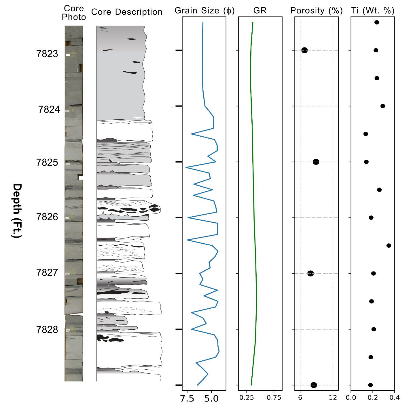
All wells in the study area have well-log data in the cored interval, ranging from having a full suite of logs (Fig. 3) to one well only having gamma-ray (S821). In cases of missing well-log data, the curve was imputed by using the scikit-learn Python package (Pedregosa et al., 2011) with a decision tree ML model using other wells that had all the logs desired (Fig. 3). This is not a replacement to collecting the full suite of well logs but allows for the ML models to be compared using the same datasets, as some models require matching and complete data. After the data was imputed, each well had the following curves: Caliper, Gamma Ray, Sonic, Spontaneous Potential, Density, Photoelectric Factor, Deep Resistivity, Density Porosity (Fig. 3). Each individual well-log curve was pre-processed on a per-well basis to normalize some of the differences between wells arising from different tools, vendors, vintages, and subsurface conditions. The well-log data were interpolated to a 0.1 Ft depth step basis to match the grain-size data we collected from the cores as part of this study. Further description of the original well-log data and the specific implementation of the log imputation and pre-processing is described in the GitHub repository (Martin, 2022).

Grain size
Most ML studies utilize subjective geologic classifications determined by geoscientists (e.g., lithofacies, systems tracts) (Hall & Hall, 2017). Our goal was to minimize the interpretive error in lithologic description, and thus grain size was determined by the authors using a grain size card and physical inspection of the core itself (Compton, 2016). While there is still human error and bias in determining grain size visually (see discussion in Jobe et al., 2021), it is more objective than interpreting stratigraphic facies or other more subjective/qualitative classifications. The grain-size data were collected using a categorical guide (e.g., upper-fine, Wentworth, 1922) and digitized and converted to the phi scale to have a linear, numeric scale (Krumbein, 1938); finally, these data were interpolated onto a 0.1 Ft scale (Fig. 4).

XRF Geochemistry
X-Ray Fluorescence (XRF) is a non-destructive measurement technique commonly used on core material to obtain efficient and accurate elemental composition (Young et al., 2016). For this study, we collected data using a Bruker Handheld Tracer 5G portable XRF every 0.5Ft on the core, using a 50kV energy level and 90 second collection time. Comparing results of the standards used before and after every day of data collection, most differences were below measurement error and therefore no corrections were needed. We used a helium purge to further enhance data quality of lighter elements such as magnesium, aluminum, and silicon. The five elements we will focus on for this study are aluminum (Al), titanium (Ti), silicon (Si), calcium (Ca), and magnesium (Mg). These five elements were chosen due to relatively higher proportion of total weight percentage, and use as a detrital indicator (e.g. Al, Ti, Si ratios). The entire elemental suite is available in the online supplementary material.
Porosity
Porosity measurements from core plugs were taken from legacy scanned PDF reports available on Wyoming Oil and Gas Conservation Commission and USGS Core Research Center websites. These data were not processed in any way to attempt to normalize for differing methodologies and standards between various laboratories, The largest potential differences are different laboratories, improved methodology with time, and the specific calculation methodology of porosity. The depths of porosity measurements were interpolated to the most reasonable decifoot (e.g., 11-12 Ft. became 11.5 feet).
Image Data
Image data were collected by the authors and by USGS core research center staff on the cores in this study (table 1). Images have various core-tray sizes, amount of core, lighting conditions, and resolution. Due to this variability, we did not employ an automated ML model to trim, edit, and stack core images into a depth registered core column (e.g., Meyer et al., 2020), but rather manually performed this task. To reduce errors from shadows and edge effects, we cropped the middle 60% of the core image for the analysis (Fig. 5). After the cropped image was manually depth registered, the standard (RGB format) images were converted to Hue-Saturation-Value values (HSV, Joblove & Greenberg, 1978; Smith, 1978) using the scikit-image package (Van Der Walt et al., 2014). This transformation reduces the differences caused due to lighting, shadows, and camera type/setup. We tested using Red-Green-Blue (RGB) channels from the original image as input features rather than HSV, and RGB did not improve results in our testing because the RGB channels are highly correlated to the value channel. The HSV values for each discretized depth step (0.1 ft, Fig. 5) are then further reduced from the entire image to median and mode of H, S, and V values, along with the inter-quartile range of saturation and value. This compresses the amount of data for each depth step by 2-3 orders of magnitude compared to full image data; similar transformations were used by Martin et al. (2021) for core image data, and in both cases allow for efficient model runtime and use of computational infrastructure.

Core to Log offset
For studies that use both core and well-log derived properties for analysis, typically a core-to-log depth shift is performed to correct wireline stretch and core loss/breakage during drilling operations (Fontana et al., 2010; Jeong et al., 2020). In this study, we compared 3 different strategies: no offset, a qualitative offset, and a quantitative offset. The no offset is a base case, where no depth shifting was done to either dataset. The qualitative depth shift was done by visually inspecting log patterns, and matching patterns. The quantitative offset utilizes a simple linear regression method to compare gamma-ray log and the grain size to further fine tune the qualitative offset to the nearest 0.1Ft. This linear regression methodology assumes that mudstones generally have a higher gamma-ray value compared to sandstones and testing shows that this method matches these well-log peaks to core-derived grain size quite well.
MACHINE LEARNING REGRESSION MODELS, EVALUATION AND PARAMETERS
Overview
This study focuses on prediction of core-derived properties using standard well-log and core-image summary data (Fig. 4, 5). We chose to explore five machine learning models, ranging in complexity from multiple linear regression to deep neural networks. The models were selected to show a range of algorithm complexity and structure. There are many ML models for supervised machine learning regression problems, but we chose models that have a Python interface, are actively maintained (i.e., public releases within the last twelve months), and have detailed documentation. There are many other models we could have chosen, and we hope other researchers will explore those models with the same dataset published with this study. A few examples of untested models are AdaBoost, LightGBM, and k-nearest neighbors, and we expect these models to perform similarly to models tested in this study. To replicate this research, the models and code are available at https://github.com/ThomasMGeo/LewisML (Martin, 2022). To install and use all code provided in the github repository, prior installation of some common Python packages is required, including Python 3.6+, Jupyter Notebooks (Kluyver et al., 2016), Lasio, Welly, Pandas (McKinney, 2010), Numpy (Harris et al., 2020), Scikit-Learn (Pedregosa et al., 2011), Scikit-Image (Van Der Walt et al., 2014), XGboost (Chen & Guestrin, 2016), Catboost (Prokhorenkova et al., 2018), and Tensorflow (Abadi et al., 2016).
Hyperparameter Tuning
Many ML models have hyperparameters that can be tuned to improve the learning process of the model (Mantovani et al., 2017, 2019). One example of a hyperparameter for XGBoost is the maximum depth of each decision tree; tuning these values often results in a lower model error compared to an untuned model (Table 2). We used a ‘grid search’ method to automatically perform hyperparameter tuning (Liashchynskyi & Liashchynskyi, 2019). Grid search is a parameter sweep method where each set of specific parameters are evaluated. While there are other methods for hyperparameter tuning, the ‘grid search’ method has built-in functionality for the five models used in this study. The bounds and hyperparameters that were tested are available in the GitHub repository (Martin, 2022).
Evaluating Regression Models
Evaluating machine learning models requires a scoring metric to evaluate model performance. To evaluate regression models, we use two main metrics: Root Mean Squared Error (RMSE) and Mean Absolute Error (MAE, equations 1 & 2 respectively). Minimizing these two error types gives insight into model ranking and performance for skewed and non-gaussian datasets common to geology. This non-linearity is also why R2 was not used, as we are comparing linear and non-linear models and datasets.
RMSE=√¯(f−o)2
MAE=∑ni=1|f−o|n
Where f is predictions, o is observations, and n is number of errors (Chai & Draxler, 2014).
Utilizing both metrics gives a more complete insight into the error structure than using one alone. There are advantages and disadvantages to both metrics (Chai & Draxler, 2014; Willmott et al., 2009; Willmott & Matsuura, 2005). RMSE tends to have better assessment of performance when errors are gaussian and is also more flexible as a distance metric compared to MAE (Chai & Draxler, 2014). This manuscript will focus on RMSE but will use MAE as a differentiator if the RMSE is very similar.
MACHINE LEARNING MODELS
Multi-variate Linear Regression
Linear regression is a data analysis method that constructs a linear relationship between n variables (Montgomery et al., 2021). There are various ways to calculate error; for this study we used least-squares (Myers, 1990). Linear regression for this study utilized multiple variables (e.g., the well-log curves in Fig. 3) and is thus termed multi-variate regression (MVR). Major advantages of MVR are its computational efficiency, model interpretability (using R2 or other metrics), and it has no need for hyperparameter tuning. One downside to MVR is the input variables need to be linear, and many geoscience relationships are non-linear; the non-linear to linear transformation creates information loss, which is sub-optimal.
Support Vector Machine
Support Vector Machine models (SVM) (Chang & Lin, 2011) have been commonly used since the 1990’s and have been used with success to model physical and earth science processes (Okwuashi and Ndehehe, 1996; Balabin & Lomakina, 2011; Bermúdez et al., 2019; Pisel & Pyrcz, 2021; and others). While SVM’s are common for classification tasks, we will be using a specific type of SVM built for regression, specifically the Support Vector Regression Machine (SVRM, Drucker et al., 1997). An advantage of SVRM is its robustness to outliers (Drucker et al., 1997), while a downside is the difficulty of scaling it to very large datasets.
XGBoost
XGBoost (Chen & Guestrin, 2016) is a gradient-boosting algorithm typically applied to decision trees (Quinlan, 1986). Gradient Boosted decision trees (GBDTs) are generally flexible for use with missing, noisy, and unscaled data. This makes them particularly useful for practical predictions on real geoscience data, although this algorithm can struggle on sparse data. XGboost has been used with great success for subsurface well-log classification tasks (Bormann et al., 2020; Dev & Eden, 2019; Hall & Hall, 2017; Martin et al., 2021).
Catboost
Catboost (Prokhorenkova et al., 2018)) is another gradient boosting decision tree (GBDT) algorithm, but with some important differences as compared to XGBoost. The ability to use Catboost with noisy, unscaled data is unchanged from XGBoost, but Catboost reformulates the specific boosting algorithm to better honor the data distributions throughout the training cycle (Prokhorenkova et al., 2018). On a range of test datasets, Catboost has shown up to 12% improvement over XGBoost (Prokhorenkova et al., 2018). Catboost has recently been used for subsurface investigations with success, particularly when compared to other methods (Tang et al., 2021; Zhong et al., 2021).
Deep Neural Networks
Deep Neural Networks (DNN) are a specific type of neural network, with many (2+) layers between the input and output layers. DNN can be used for either classification or regression on nonlinear data types and perform best with large (n > 100,000) datasets. One downside to DNNs is the lack of interpretability (i.e., feature importance, hyperparameters) compared to other ML methods like decision trees. DNNs have been used successfully for geologic image recognition and classification problems (Jeong 2020; Chawshin et al., 2021; Lauper et al., 2021; Martin et al., 2021; Meyer et al., 2020; Falivene et al., 2022). DNN regression has also been used to estimate river sediment yield (Cigizoglu & Alp, 2005). The DNN in our study is two layers, with further model parameters available on the GitHub (Martin, 2022).
K Means Clustering
While this study is generally focused on regression-based prediction, the XRF data collected from the cores is quite useful for constraining basin evolution as well. Because multiple clinothems were sampled in varying spatial locations (Fig. 2), we chose k-means clustering to find similarities in the XRF data, which include ratios and amounts of specific elements. K-means clustering (Arthur & Vassilvitskii, 2007) is an unsupervised ML method that organizes data into clusters of similar data around a centroid. K-means algorithm minimizes the average squared distance between an observation and a cluster, while continually testing out new centroid locations until the optimum locations are discovered. One advantage and disadvantage to k-means is that the number of clusters must be chosen by the user. The advantage of a user defined number of clusters is you can match the same number to number of facies or other geologic classification scheme, but the disadvantage is that this selection can promote bias. K-means is also generally computationally efficient compared with supervised ML methods and does not require hyperparameter tuning.
RESULTS
Grain size
Table 2 shows the results for the five ML models predicting grainsize using well-log data (Fig 3.) reporting both RMSE and MAE, for each core-to-log offset. The two models that had the lowest RMSE were both gradient-boosted decision trees (GBDT), XGBoost and Catboost respectively. These two models had very similar results, but XGBoost with hyperparameter tuning had the lowest error for both RMSE and MAE for all core-log offsets (Table 2). The overall median error for all models was the lowest for quantitative offset compared to the qualitative and no offset cases. XGBoost had the lowest RMSE on the quantitative offset with an RMSE of 0.67. Deep neural networks performed similarly to SVRM. All models improved on multi-variate linear regression results.
Using core image data alone did not improve the ability to predict grain size demonstrably compared to the well log data with Catboost, as shown in Table 3. Combining both the well-log and core-image data also did not result in a significant decrease in RMSE or MAE compared to well-log data only. Issues with lighting, crack detection, and similar coloring of the different lithologies (specifically in the E997 core) were insurmountable for the ML model. We tested various pre-processing pipelines to help eliminate these issues (e.g., variable lighting and legacy photo types) without success. Future core-image studies should prioritize even and normalized lighting during data acquisition (cf. Martin et al., 2021).
Porosity
Table 2 shows the results for the four ML models, reporting both RMSE and MAE, for each offset on predicting plug-derived porosity measurements from well-log data (Fig. 3). The error did not reduce between the no offset to qualitative offset, but the quantitative offset had the best performance out of the three offsets. Along with GBDT, the SVRM performed very well for the qualitative offset, but not on the other two offsets. Deep neural networks were not utilized for porosity due to the small dataset size. E997 is a ‘behind-the-outcrop’ core, and the shallowest core in the dataset with porosity data. Due to the non-stationarity of these porosity data points for deeper and more relevant subsurface conditions, E997 was not used for testing or training datasets. Testing also revealed that including E997 resulted in a higher RMSE.
XRF elemental data
Table 2 shows the results for the five ML models predicting XRF measurements, reporting both RMSE and MAE, for each offset from well-log data (Fig. 3). XGBoost had the lowest (best) RMSE for each offset, with SVRM and Catboost with the second-best results, respectively. The DNN results are similar with the multi-variate linear regression results. The overall median was relatively similar between all offsets, but the qualitative offset had the lowest RMSE. Catboost had the lowest RMSE overall, with a combined RMSE of 1.00 of the five element panel (Al, Ti, Si, Ca, Mg) using the quantitative offset.
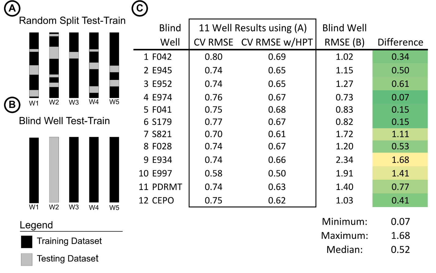
Test-Train Splits: Random Split vs. Blind Well
Figure 6C highlights the results for predicting grain size using Catboost, comparing the error from randomly test-train splitting of the dataset vs. using a single blind well as the test split (Fig. 6A-B). On the randomly split dataset, 25% of the data is held out for testing. Figure 6A illustrates visually how this is implemented. Using the RMSE from the randomly split testing dataset is overly optimistic (ie lower, column 3, Fig 6C) for each of the tests compared to the blind well, with the minimum RMSE increase of 0.05, the maximum of 2.02 and the median difference of 0.58 (Fig. 6C). This is only for one core-log offset and one ML model but highlights the possible variability in prediction results using different test-train split methodologies.

DISCUSSION
1. Machine Learning Model Selection
**_xrf_cross_plots_comparing_calcium_(ca)_to_silicon_(si)__and_sulfur_(s)_to_iron_(fe).tiff)
Many studies have focused on the best approaches and models for well-log classification and regression tasks, with gradient-boosted decision trees (GBDTs) commonly being the most effective models (Bormann et al., 2020; Hall & Hall, 2017). Our study generally confirms this, with Catboost and XGBoost occupying the first- or second-best model type <80% of the time and scoring as the winners of both the SEG 2016 and FORCE 2020 well-log classification contests (Bormann et al., 2020; Hall & Hall, 2017). GBDTs are generally flexible to missing and unscaled data and can be trained on a relatively small amount of data compared to a DNN due to model architecture. While each data type and offset had a ML model with the lowest error, the difference between the first-place and the second-place model is generally very small (1-5%, see Table 2). These differences have a minor impact on final interpretation and utilization, so a ML model that is easier to implement and interpret may be preferred even if it is slightly less accurate. For example, while SVRMs have low error with smaller datasets, they are slower to train, and require more specific pre-processing compared to gradient boosted decision trees due to model architecture. Due to these reasons, a GBDT (Catboost, XGBoost) would generally be preferable. For this dataset, a second- or third-place decision-tree model has significant benefits over MVR due to the need to linearize MVR inputs. For subsurface investigations using well-logs, MVR is a useful baseline comparison due to computational efficiency and interpretability, but using MVR alone will generally underperform compared to other ML methods because well log data often have non-linear distributions.
While DNNs are popular for a variety of deep learning tasks, including image recognition, none of the DNN models had the lowest error in this study (Table 2). This poor performance, paired with a lack of clear interpretability suggests that DNNs are not recommended for datasets of this size, as larger, higher dimensional datasets might have increased performance using a DNN where interpretability is not a main factor for evaluation or use. For well-log analysis and prediction, DNN class of models would need a specialized dataset or research question to take advantage of the inherent model complexity and infrastructure. While further research will continue to refine which models and class of models have the best performance, future needs for most geoscience professionals will include easier model deployment, interpretation, and dataset augmentation (Burkov, 2020; Curtis et al., 2020; Jahic et al., 2019; Molnar, 2022). Future researchers can build on the results this study to improve ML model parameterization and deployment practices.
2. Core Image Data
While core-images have been used for classification of facies and lithology primarily using DNNs, image-based ML methods require substantial computing resources (Chawshin et al., 2021; Jeong et al., 2020; Lauper et al., 2021; Martin et al., 2021; Pires de Lima et al., 2019; Solum et al., 2022; Zhang et al., 2021). Generally, these DNN workflows are used on well curated datasets with standardized core imagery (e.g., Martin et al., 2021). However, the core photographs in this study are more variable (e.g., various cameras, formats, resolutions, and lighting conditions). For example, the core images in this study had visible dust, debris, labels, and other surface imperfections. Lighting is also generally inconsistent, causing variations in the HSV value from the top to the middle of the core boxes. The core-image data underperformed compared to other data types in this study, perhaps due to this image-quality variability. Furthermore, while some studies have had success using color to predict lithology (e.g., Martin et al., 2021), color alone is not diagnostic of grain size. For example, the E997 core has dark grey mudstones but also mudstones that are light grey in color, similar to the color of sandstone in this specific core (Fig. 4). Physical inspection of the core makes differentiating between grain sizes straightforward rather than relying on photographs alone. These issues emphasize the need for high resolution, depth-registered, fit-for-purpose core photography (e.g., using methods of Meyer et al., 2020), preferably paired with another sensor type (hyperspectral, XRF, LiDAR) to differentiate between differences in lithology, grain size, and other useful geological indicators.
3. Test-Train Splits: Blind-Well Splits Honor Traditional Geoscience Workflows
Randomly splitting datasets into testing and training sets is common in ML research, especially for data consisting of independent measurements (e.g., image datasets, web traffic). However, in the geological realm and particularly with borehole-based datasets, some of the measurements are correlated to each other and thus dependent. However, the identification of geologic parameters from well-logs is non-unique, thus calling into question the concept of random test-train splits.
Blind predictions (e.g., predicting facies in a new well location) is needed for most geoscience applications. Using random test-train splits with multi-well datasets (e.g., Fig. 6A) is still a valid way to test and verify ML modeling approaches and can be useful for specific well-based workflows such as predicting missing core data, confirming data quality, verifying previous interpretations, or other specific needs. However, the results from random, inter-well testing and training datasets will be overly optimistic on blind wells (Fig. 6) because every well (and corresponding well log) has different data conditions (age, wireline contractor, pressure, equipment, size, etc.) We expect slight changes within the Dad Sandstone facies during basin evolution, but it is the choice of the modeler to decide if the dataset has stationarity, and if the test-training splitting methodology is appropriate. For this study, the core dataset encompasses a wide range of Dad Sandstone facies due to the spatial and age variability of the wells we chose (Fig. 1C), and therefore we assume stationarity. But with these model types, extrapolating outside the range of test data is not recommended.
One potential issue with applying this methodology to other formations is increased complexity and heterogeneity within one formation compared to the Dad Sandstone/Lewis Shale. Mixed carbonate and siliciclastic deepwater systems have centimeter-scale geochemical and facies changes, which may affect model performance as compared to this study. Some formations will need to be split into sub-regional areas or temporal zones to maintain stationarity depending on research questions and dataset quality/quantity. While using ML can be a data-driven approach, many of the decisions done before a ML modeling workflow are subjective, but important decisions that require geoscience domain knowledge. Another reason for inter-well underperformance is that each well generally has different vendors collecting the downhole data, vintages, reservoir conditions, depths, and other variables that make it more difficult for the data to be directly transferrable between wells. With a more modern, curated dataset, the differences would potentially be smaller than results presented in this study.
Future work exploring multiple facies in a single well-log, or other stacked succession multi-classification research might require different model types (Long short-term memory, convolutional neural networks, etc.). These types of models use the context above and below the region of interest for classification (e.g., Martin et al., 2021) and are well-developed due to research for audio and time-series analysis. These model types also require full sequences of data and would not perform well with randomly split datasets. Exploring these model types and relating them to geological processes and the completeness of the stratigraphic record (e.g., Sadler, 1981) is an exciting area of future research.
Whichever method is used for splitting data into testing and training datasets, it is important to describe the specific workflow that was performed, ideally with the release of code (e.g., Martin, 2022) so that the work is reproducible for future ML research. These details could have an outsized impact on how the results from ML workflows would be generalizable and transferrable to truly blind data (Fig. 6).
4. Implications for chemostratigraphic heterogeneity prediction
While ML models can predict elemental data from well-log data (with a degree of error and uncertainty), the results presented in this study do not replace the need for original data collection for research questions focused on chemostratigrapic patterns and processes in deep-water systems, which are highly variable both spatially and temporally (i.e., in depth), and can change within centimeters. A limitation of this dataset is that XRF measurements were only collected every 0.5 Ft (15.24 cm), which cannot resolve the true lithologic and geochemical variability that is seen in core photos (Fig. 4).
We assume stationarity in the XRF data from the entire twelve-well dataset, a reasonable assumption for most practitioners because the data is within the same formation within the same basin. Exploring the k-means clustering results (Fig. 7) shows a spatial pattern for the sandstone samples, organizing into three groups that are geographically consistent (Fig. 7B). These clusters correlate with time of deposition as well, as the basin was filled north to south (Fig. 2; Carvajal, 2007; Carvajal & Steel, 2006; Koo, 2015). We tested various combinations of XRF elemental data as inputs to the k-means clustering algorithm, and the trends in Figure 7 were consistent with multiple experiments. The change in sandstone bulk geochemistry could be caused by temporal changes in source provenance, sediment routing, or diagenetic differences (e.g. Hunt et al., 2015). The basin sediment was primarily sourced from the north, but also had input from the west (Rock Springs Uplift, Hettinger & Roberts, 2005). Foreland basins commonly show temporal variability in transverse and axial sediment sourcing that affect sandstone composition (Koshnaw et al., 2020; Malkowski et al., 2016; Primm et al., 2018; Sharman et al., 2018; Szwarc et al., 2015), and the Green River Basin may have had temporal changes in the three dominant source areas (Wind River Range, Granite Mountains, Rock Springs Uplift, Hettinger & Roberts, 2005). However, untangling these relationships for our dataset and basin modeling would require additional datatypes (e.g., detrital zircon data) and sample locations throughout the basin, compared to our single North-South transect (Fig. 1). Different present day burial depths (~500 ft. for E997 to 13,000 ft. in the south) could also impact the differences we see today due to differential diagenesis.
The mudstone XRF data do not show strong spatial and/or temporal trends with the available geochemical data. Using k-means clustering with 2, 3, 4, and 5 clusters, none of the resulting clusters were geologically meaningful in either relative age or location within the basin (Fig. 7). Changing the element and element ratios used in the clustering experiments significantly affected the cluster results; the results shown in figure 7B is just from one set of feature inputs. We attribute the lack of strong spatiotemporal clustering in mudstone XRF data to be related to (1) the relative ease of basin-wide mud transport in marine depositional systems as compared to sand (Drake et al., 1978), (2) a more consistent mud provenance through time (cf. Fildani & Hessler, 2005), (3) sub-regional diagenetic and anoxia changes that affect mudstone geochemistry more than sandstone. However, there are minor differences in mudstone elemental data through time that were not revealed in the clustering results. For example, the relatively enriched sulfur and calcium for the MFS 5-8 group suggests a more anoxic environment during time of deposition (cf. Dijkstra et al., 2016) as compared to the older and younger intervals (Fig. 7). This difference might be driven by being on the edge of the basin compared to the more central sediment fairway (F028, E934, E997, eastern edge of basin). Additional data in the center of the basin may shed light on these hypotheses, helping to improve our understanding of basin circulation dynamics and geochemical evolution. To capture finer-scale detail and vertical heterogeneity, a core-scanning workflow that collects depth-continuous data (e.g., Birdwell et al., 2020) would be useful, and future work could compare results from a core scanner to the hand-held XRF data collected in this study.
5. Implications for stratigraphic heterogeneity prediction
This study provides a workflow and best practices to predict properties, including grain size, from well-log data. But grain size alone is not indicative of depositional process, sub-environment (levee, channel, lobe), level of confinement, and other stratigraphic information needed to make a holistic interpretation. We propose that this work should be used in conjunction with other more conventional interpretation methods (e.g., graphic logging, facies classification) and other ML workflows to further constrain reservoir and geologic properties. For example, the ML workflow described here could be used to generate initial results for a basin-wide study focused on sediment routing and chemostratigraphy, upon which more detailed, bespoke studies could provide more accurate information about depositional sub-environments, depositional processes, chemofacies, and diagenesis.
CONCLUSIONS
This study utilizes a newly digitized twelve-well dataset from the Dad Sandstone Member of the Lewis Shale in the Greater Green River Basin, Wyoming to evaluate performance of five machine learning models and workflows to predict common core-derived properties from well logs and core images. The overall best performing models with the lowest RMSE are gradient-boosted decision trees (XGBoost, CatBoost). These types of ML models are especially useful for geoscience problems, as they can handle both regression and classification while being less sensitive to unscaled, missing, and noisy data. For example, utilizing CatBoost model to predict grainsize, using well-log data the RMSE is 0.75 which is below the 5-model median RMSE of 1.00. Using core image data performed worse, with a RMSE of 1.13. The core-image regression result emphasizes the requirement to use high quality, fit for purpose core image data with consistent lighting. Core imaging in the future should be treated as a potential digital data type, and not just as a storage bookkeeping activity. The XRF data also yielded insights into basin evolution with the sandstone showing a strong spatiotemporal organization into north, central, south groupings, while the mudstones show a more mixed depositional pattern. This might be due to diagenetic, mixing, or other geochemical differences during time of deposition.
While the models developed in this study can predict grain size, XRF elemental measurements, and porosity (with a certain amount of error) from well logs and core images, this does not negate the need to collect more data in the future for other Dad Sandstone datasets, and other, more general deep-water stratigraphy datasets. More data would allow for better quality control of the specific ML research question, and confirmation that the models perform on a satisfactory level. The detail provided by predicted grain size every 0.1Ft is not the same level of detail as physical core inspection and description done manually by a trained sedimentologist (Fig. 4), which will still be needed as ML models are improved and refined for geoscience applications.
This research demonstrates the possibility of predicting both inter-well and blind-well core-derived reservoir properties from well logs and core images using fully open-source Python packages (Martin, 2022). Utilizing a blind well testing strategy compared to a random split will have large differences on results depending on use case. We recommend using blind-well holdouts for the majority of geoscience uses, as even for inter-well training and testing it will still be a valid measure of error. The research presented here will also guide further ML model choice for geoscientists and researchers alike. This workflow can be scaled from twelve wells in south-central Wyoming to thousands of wells with digital well-log data worldwide.
ACKNOWLEDGMENTS
We acknowledge the funding support from Chevron Center of Research Excellence (core.mines.edu) at Colorado School of Mines and Rocky Mountain Association of Geologists Cluff Scholarship. Nigel Kelly and Jonathan Knapp at Bruker Corporation (https://www.bruker.com/) assisted with XRF equipment and data-processing. USGS staff at the Core Research Center (https://www.usgs.gov/programs/core-research-center) helped with core handling and data curation. Reviews from Ellen Wersan and two anonymous reviewers greatly improved this manuscript.