
INTRODUCTION
Sedimentary deposits are important records of planetary surface evolution, but exactly how deposits represent their ancient environments is not fully understood. The continuity of time in the sedimentary record is remarkably low in vertical sections (Jerolmack & Sadler, 2007; Sadler, 1981; Sadler & Jerolmack, 2015). The poor representation of time has been often attributed to the sedimentary record’s propensity for recording significant and relatively rare scour-and-fill events. For instance, steadily accumulating fluvial strata might be episodically eroded and rapidly replaced during major floods (Ager, 1993), a behavior that has been recreated in physical experiments (Barefoot et al., 2021; Leary & Ganti, 2020). However, many sedimentary deposits do not seem to have accumulated during such high-magnitude events, and instead represent relatively common sediment transport conditions (Paola et al., 2018). Further, hiatus in deposition is perhaps the most important time-sink in the sedimentary record, not requiring the significant removal of deposits to explain time gaps (Miall, 2015).
The presence of depositional hiatus and preserved strata representing common flows can both be attributed to the relief of depositional systems. Local relief is capable of driving rapid sedimentation rates that lead to nearly fully preserved deposits, with local referring to a scale similar to the feature in question (Ganti et al., 2020; Miall, 2015; Reesink et al., 2015). For example, dunes with fully preserved stoss and lee slopes have been identified buried beneath the bars they accumulated in front of (Reesink et al., 2015). At less extreme levels of preservation, bar topography can still drive rapid dune aggradation in front of bars (Cardenas et al., 2020; Lyster et al., 2022). Fully preserved bars can similarly be found in strata, preserved within ancient channel topography (Cardenas et al., 2020; Chamberlin & Hajek, 2019; Mohrig et al., 2000). These sources of relief are generated morphodynamically, in that their formation occurs from the interactions of fluid flow, sediment transport, and evolving topography, and requires no external forcing.
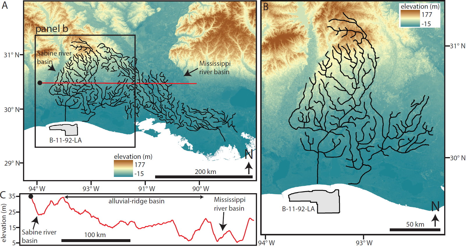
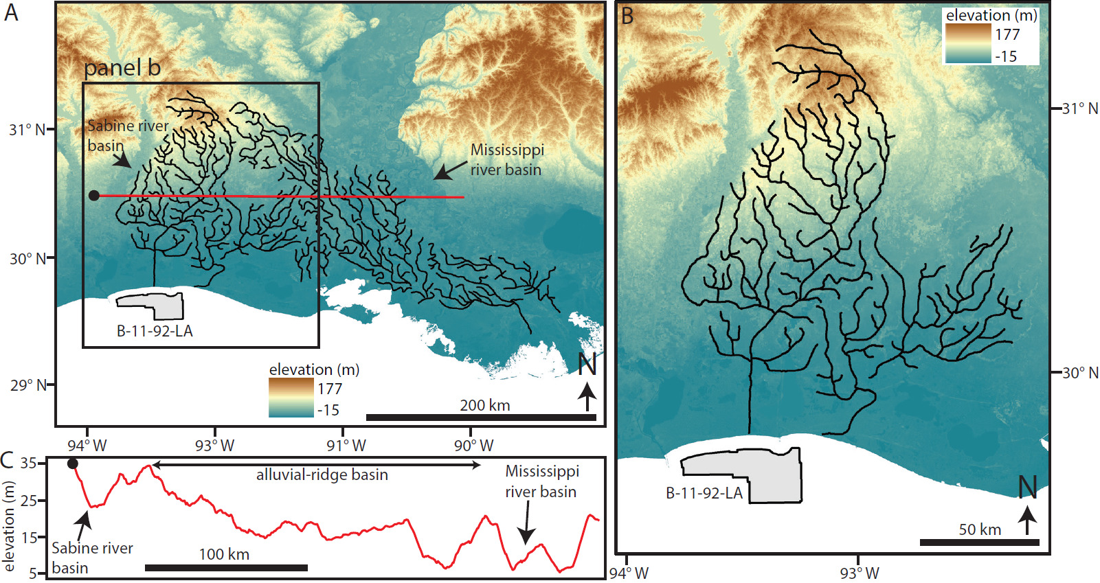
A larger source of morphodynamic relief may be preserving fluvial channel belts, similar to the way bar topography preserves dunes and channel topography preserves bars. This is generally predicted by theory showing morphodynamic feedbacks can occur up to the 100s of km-scale in fine-grained sedimentary systems (Ganti et al., 2014). Channel belts in the subsurface US Gulf Coast imaged in 3D seismic reflectance volumes show minimal signs of reworking, despite estimated subsidence rates that suggest the time required to accumulate a channel-belt thickness of sediment is much greater than the time required for a channel to avulse, re-occupy a location, and rework older channel belts (Paola et al., 2018). That is, sedimentation at subsidence rates alone would be unable to fully bury channel belts and protect them from scour by younger channels. Minimal reworking coupled with the order of magnitude difference between avulsion frequency and subsidence rates indicate that depositional hiatus was an important part of this stratigraphy, during which channel and floodplain deposition shifted laterally (Paola et al., 2018). With sedimentation rates on floodplains being a function of distance from the channel (Pizzuto, 1987), the highest elevations on alluvial plains are often located along channel margins (Hassenruck-Gudipati et al., 2022), forming topographic features containing channels called alluvial ridges. This lateral variability in sedimentation builds relief, developing basins which channel belts can be routed into (Aslan & Blum, 1999; Speed et al., 2022; Swartz et al., 2022). These alluvial-ridge basins often develop well-defined tributary drainage networks despite their relatively low relief (Swartz et al., 2022; Fig. 1).
Indeed, 1D core data suggest that channels are often steered into these depressions following the abandonment of a higher, perched channel (Aslan & Blum, 1999). High-resolution 2D seismic reflectance images have shown that channel belts preserved within these basins can have fully preserved point-bar rollovers, consistent with the preservation of nearly the full vertical extent of the channel belt (Speed et al., 2022). Numerical models of alluvial-channel aggradation and avulsion show similar routing (Jerolmack & Paola, 2007). This general process, whereby the topography associated with a channel steers later channelized deposition into topographic lows, is called compensational stacking (Straub et al., 2009).
We hypothesize that coastal basins between alluvial ridges are the source of morphodynamic topography preserving channel belts. Here, we used a 3D seismic reflectance volume imaging channel belts to further test this hypothesis using measurements that took full advantage of the three dimensionality of the data, adding significant spatial coverage to very local but high-resolution 1D and 2D datasets supporting the hypothesis (Aslan & Blum, 1999; Speed et al., 2022). The volume images Pleistocene alluvial strata offshore the US Gulf Coast. Late Pleistocene sea-level lowstands are recorded by coastal plains that pushed farther into the Gulf of Mexico than in the modern and the cutting of incised valleys (e.g. Galloway et al., 2000, 2011; Simms et al., 2007). These Pleistocene coastal plains and valleys are buried and filled by younger deposits accumulated since lowest sea level (Meckel & Mulcahy, 2016; Speed et al., 2022).
METHODS
To test the hypothesis that alluvial-ridge basins preserve fluvial channel belts, we acquired a 3D seismic volume imaging channel belts, and mapped the basal and lateral extent of the belts. From this mapping, we generated geometric measurements of the belts and checked (1) if channel belts have a spread of orientations consistent with steering by coastal alluvial-ridge basin topography, which would be expected if Pleistocene alluvial-ridge basins were generally similar to the modern in terms of size and shape, and (2) if channel belts are preserved without significant reworking over 10s of km, or many times their width.
We downloaded 3D seismic reflection volume B-11-92-LA imaging offshore Louisiana from the United States Geological Survey’s National Archive of Marine Seismic Surveys (USGS NAMSS). This volume was collected in 1992. We used a subset of the volume covering 379 km2 centered on a location about 16 km offshore Louisiana (Fig. 1), with 20 m bin spacing and 4 ms sampling rate. In the shallow interval of interest, the dominant frequency was 38 Hz and P-wave velocities were assumed to range from 1,900 m/s to 2,700 m/s (e.g., Armstrong et al., 2014; Straub et al., 2009), leading to a best-case vertical resolution of 6 to 18 meters with better detection limits. The resolution precludes an accurate measurement of channel-belt thickness, but the lateral continuity of channel belts thinner than the resolution limit helps with the detection of their basal scour surfaces (Zeng, 2018; Zeng et al., 2020). This study was purposely restricted to the first 1,000 ms of acoustic wave two-way-travel time (ms TWT) because it had the highest frequency content for the reflected acoustic waves and afforded the best possible resolution of imaged strata. We estimated that 1 ms TWT represents from 0.8 m to 1 m, based on fossil studies performed in the region (Armstrong et al., 2014; Hentz & Zeng, 2003).
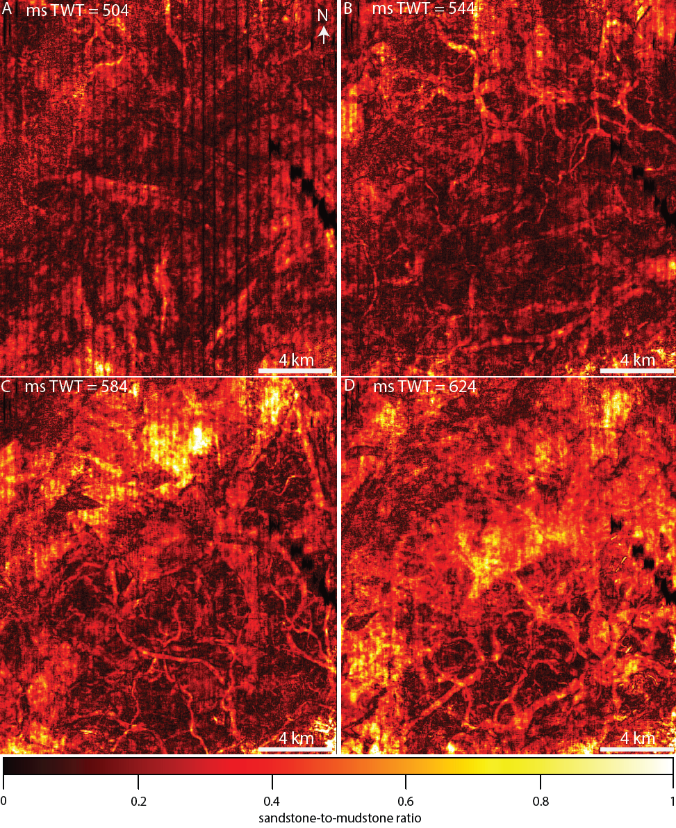
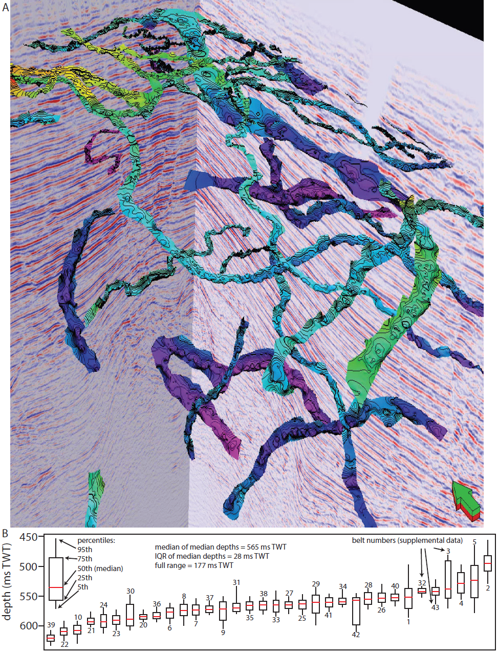
We identified and mapped channel belts in the software Petrel. We used a combination of amplitude cross sections and variance and sweetness horizontal slices, taking advantage of the Link Cursor toolbox to help match features between windows. Amplitude volumes are higher resolution and useful for mapping in vertical sections, while horizontal slices through variance volumes accentuate the edges of channelized features (Bahorich & Farmer, 1995; Liu & Marfurt, 2007) and sweetness provides a qualitative constraint on the ratio of sandstone vs. mudstone that is useful for identifying channel belts (Fig. 2; Hart, 2008a, 2008b). We first mapped the basal scour surfaces using arbitrary cross-sections oriented perpendicular to the channel belt as seen in horizontal slices. We then outlined channel belts in horizontal slices using the Create Polygon tool. Using the Surface tool, we generated a surface fit to the mapped basal scours within the lateral bounds of the horizontal polygon. Using the Points tool, we converted the basal surface of each channel belt into a series of points spaced 20 m apart, and extracted subsurface depth in ms TWT at each point, giving each channel belt a distribution of subsurface depths. Throughout, we refer to channel-belt depths as a belt’s vertical position beneath its basal surface.

Mapping the horizontal polygons in Petrel is necessary to set the extent of the basal scour surfaces, but ArcGIS facilitates more careful horizontal mapping with the use of a drawing screen. We imported the horizontal polygons and selected sweetness horizontal slices into ArcGIS to guide our mapping of the lateral extent of the channel belts (after Alqahtani et al., 2015, 2017). We separately mapped the long edges of each channel belt. We used the Generate Points Along Lines toolbox to generate points along each edge with real X and Y coordinates.
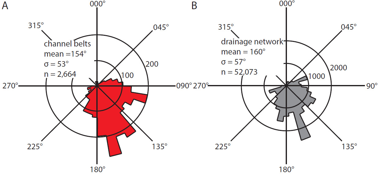
We imported channel-belt-edge coordinates into Python and wrote scripts that used these coordinates to measure widths, centerline orientations, and channel-belt lengths. We calculated channel-belt widths by comparing the distances between points on opposite edges of the same channel belt. On one edge, our script went through every point, measuring the distance to every point on the opposite edge. We defined a local width measurement as the shortest distance to a point on the opposite edge, and measured a width for every point along one belt edge. We used the median width as the representative width for the belt, and reported the standard deviation. To generate a centerline, we took the average X and Y coordinate from points used to measure width. This generated unevenly spaced points, which we imported back into ArcGIS and used in tandem with the mapped edges to guide manual mapping of a centerline, which we then converted into a series of points spaced 100 m apart. In Python, in order to generate rose diagrams defining belt orientation, we used a script that calculated the azimuth direction between centerline points in the general downstream direction, giving each channel belt a number of measurements equal to the number of points defining its centerline (after Cardenas & Lamb, 2022). We calculated channel-belt lengths as the number of points defining a centerline multiplied by the spacing, 100 m, and calculated sinuosity as the channel-belt length divided by the distance between centerline endpoints. To compare with the channel belts, we similarly measured the orientation of the modern coastal drainage network located near the seismic volume (Fig. 1B). We used channel centerlines downloaded from the USGS National Hydrography Dataset (e.g., Swartz et al., 2022, their Fig. 1).
RESULTS
We identified, mapped, and measured the stratigraphic positions and geometries of 34 channel belts. The distribution of subsurface depths along the basal scour surfaces has significant overlap at all percentile ranges (Fig. 3). We took the median subsurface depth of a channel belt to be its representative depth. The median of all representative subsurface depths is 565 ms TWT for all channel belts (452- 565 m), with an interquartile range (IQR) of 28 ms TWT (22-28 m) and a full range of 126 ms TWT (101-126 m thick). The thickness of the channel-belt interval, defined as the shallowest 95th percentile measurement of all channel belts to the deepest 5th percentile measurement, is 177 ms TWT (142-177 m).

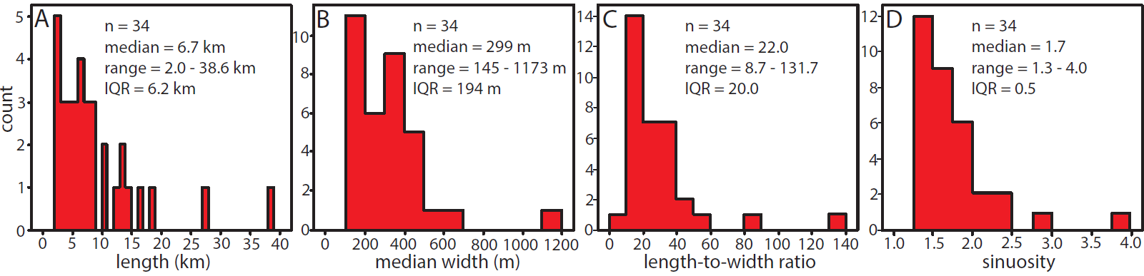
Channel-belt lengths range from 2.0 km to 38.6 km, with a median of 6.7 km and an IQR of 6.2 km (Fig. 4). Representative channel-belt widths, defined as the median width of a belt, range from 145 m to 1169 m, with a median of 299 m and an IQR of 194 m. Length-to-width ratios range from 8.7 to 131.7, with a median of 22.1 and an IQR of 20.0. Belt sinuosity ranges from 1.3 to 4.0, with a median of 1.6 and an IQR of 0.5.
__median_widths_(b)__lengt.png)
The mean channel-belt orientation is towards 154°, with a standard deviation of 53°. This is similar to the orientation of drainage channels in the modern alluvial-ridge basin, which have a mean downstream orientation towards 160° with a standard deviation of 57° (Fig. 5). Some measurements exceed ±90° from the mean. Though we find them comparable with means and standard deviations within a few degrees of each other, a two-sample Kuiper statistical method, designed to test for similarity between circular distributions, rejects the distributions as the same in their original orientations and when rotated by their mean values (p < 0.05).
We did not identify a larger-scale container for these channel belts in this, or any, interval of the volume that might be interpreted as the boundaries of an incised valley (Alqahtani et al., 2015; Simms et al., 2006). We also did not identify any tributary networks within our studied interval, which commonly develop in modern alluvial-ridge basins (Swartz et al., 2022) and which have been identified in channel-belt intervals using higher-resolution volumes (Darmadi et al., 2007; Miall, 2002; Reijenstein et al., 2011; Speed et al., 2022).
DISCUSSION
Here, we interpret the depositional setting of mapped channel belts as a Pleistocene coastal plain. We then present evidence that the belts were deposited in, steered by, and preserved within alluvial-ridge drainage basins.
Depositional setting
We interpret the lack of a clear incised valley to indicate these channel belts were instead deposited on a coastal plain. With the representative subsurface depth ranging from 452-565 m, a representative age is anywhere from 0.4 Ma to 2 Ma, or sometime during the Pleistocene (Hentz & Zeng, 2003; Straub et al., 2009). This is consistent with paleogeographic maps of the region that show Pleistocene coastal plains extending further south than the modern shoreline (Galloway et al., 2000, 2011).
The lack of draining tributary channels associated with the channel belts is not necessarily inconsistent with the alluvial-ridge drainage basin hypothesis. Though alluvial-ridge drainage channels are imaged in higher-vertical-resolution chirp volumes (38 Hz in this study versus 700-12,000 Hz in Speed et al., 2022), the lower vertical resolution of the volume used here may not be able to identify them. This may be particularly true given that the drainage channels are likely to become mud-filled, creating acoustically transparent mud-on-mud contacts. Though the identification of such channels would most directly confirm the hypothesis that alluvial-ridge basins act to preserve channel belts, we must instead test the hypothesis using preserved channel-belt orientations and geometries.
Indicators of channel-belt deposition within alluvial-ridge drainage basins
Channel-belt orientations are consistent with deposition within alluvial-ridge basins. We assume that the distribution of drainage channel orientations we measured reflects the topography of the basin (Fig. 5). The spread may indicate that the steepest slopes are not always locally oriented directly south towards the modern shoreline. While we do not interpret the ancient channel belts to be the same types of drainage channels, we do hypothesize that the channel belts were steered by the same sort of basin topography. Thus, we interpret the similar orientations of ancient channel belts and modern drainage channels, to within a few degrees for both means and standard deviations (Fig. 5), to indicate that the channel belts were deposited within alluvial-ridge basins. The relatively low sinuosity of the channel belts also suggests this distribution of orientations is driven by basin topography rather than local meandering, which is not necessarily captured by these centerline measurements (Fig. 4). This similarity of the means may also indicate that the paleoshoreline downstream of the channel belts was aligned as it is today, but further towards the south. However, the lack of exact statistical similarity between the distributions likely captures differences resulting from the drainage channels completely capturing the topography of a single basin, and the channel belts incompletely representing the topography of dozens of stacked basins, which we discuss later.
Channel-belt geometries may be consistent with deposition within alluvial-ridge basins. The preserved belt lengths of several km to 10s of km, or tens to over one hundred times belt width, seem to represent a level of continuity that would not be expected with a setting prone to significant reworking, which would shorten and amalgamate channel belts. It may be interpreted that these preserved lengths are to be expected of well-preserved channel belts, given that alluvial-ridge basins are known to preserve channel-belts vertically nearly fully (Speed et al., 2022). Though many compilations include widths and thicknesses (Gibling, 2006; Jobe et al., 2016, 2020), we are not aware of published lengths of ancient channel belts that are known to have not accumulated within such basins, which we would ideally compare our measurements to. As such, our measurements may provide a baseline for future comparisons. We note that many physical experiments which did not produce topography akin to alluvial-ridge basins do describe rapid channel reworking (e.g., Carlson et al., 2018; Piliouras & Kim, 2019; Wickert et al., 2013).
In addition to orientations, we interpret the overlapping subsurface depth ranges of channel belts to represent compensational deposition (i.e., shingling), as expected in alluvial-ridge basins (Fig. 3). If channels are being steered into relative low points following avulsions, channel belts may have significant overlap in stratigraphic position despite being of different ages. This vertical mismatch between age and stratigraphic position should be expected along the US Gulf Coast, where the relief of alluvial-ridge basins exceeds the depths of some of the largest channels (Swartz et al., 2022). If alluvial-ridge basin relief was similar in the Pleistocene, then it could explain the channel-belt scale lateral shingling and belt continuity shown here and by others (Paola et al., 2018). This sort of shingling, driven by lateral variability in basin-scale sedimentation, is often required to maintain sediment mass balance in source-to-sink sediment flux calculations, and is an important line of evidence for the prevalence of hiatuses in the sedimentary record (Jerolmack & Sadler, 2007; Miall, 2015; Sadler & Jerolmack, 2015).
The channel belts in this volume may represent the shingling and stacking of belts in anywhere from 14 to 25 distinct basins. With the channel-belt interval being between 142 and 177 m thick, if we assume Pleistocene alluvial-ridge basins were similar in relief to the modern (about 7 – 10 m deep; Swartz et al., 2022), then the belts in the volume must represent this process of alluvial-ridge basin creation and filling many times over, indicitating it is a common process in coastal alluvial settings. It is not clear whether preservation in alluvial-ridge basins must occur within a coastal backwater zone. Sedimentation patterns in the backwater zone favor aggradation and ridge development rather than lateral migration (Hudson & Kesel, 2000; Mason & Mohrig, 2018; Smith et al., 2020), but fluvial megafans develop similar alluvial-ridge topography without a downstream water body (Martin & Edmonds, 2022). That is, the routing of channel belts into alluvial-ridge basins may not be rare, but quite common across alluvial settings.
Morphodynamics in the sedimentary record
Morphodynamic processes arising from the naturally occurring interactions between flow, sedimentation, and topography play an important role in defining the architecture of the fluvial sedimentary record (Ganti et al., 2020; Hajek & Straub, 2017), and can even overwrite some external forcings (Jerolmack & Paola, 2010; Straub et al., 2020). Architecture controlled by morphodynamic processes can be observed from the bedform scale (Jerolmack & Mohrig, 2005; Lyster et al., 2022; Reesink et al., 2015) to, as we demonstrate here and as others have, the channel-belt scale (Aslan & Blum, 1999; Mohrig et al., 2000; Speed et al., 2022). The topographic relief associated with the morphodynamic preservation of channel belts is present, and even exaggerated, in subaqueous settings (Jobe et al., 2020) and perhaps even across planets. Fluvial channel belts exposed at the surface of Mars can be mapped for 10s and even 100s of km (Davis et al., 2019; Hughes et al., 2019; Williams et al., 2013), likely due to the extent of their initial preservation followed by the relative gentleness of their exhumation (Burr et al., 2009; Cardenas et al., 2022). In outcrops at Aeolis Dorsa, Mars, with depositional settings interpreted as coastal, stacking and shingling at the channel belt and lobe scales are common (Cardenas & Lamb, 2022; DiBiase et al., 2013; Hughes et al., 2019). In the Hellas basin on Mars, exposures may have an architecture more consistent with reworking, with highly amalgamated fluvial strata (Salese et al., 2020).
Given the pervasiveness of morphodynamic control on stratal architecture, we suggest that external forcings on fluvial architecture at the channel-belt scale may be identified by their interruption of morphodynamic preservation. For instance, recent work demonstrated that a lack of fine sediment supply, an external forcing driven by the lithology of the sediment source, can drive greater channel amalgamation and decreased preservation (Chamberlin & Hajek, 2022). The lack of fine sediment may have ultimately starved levees and floodplains of the sediment required to build alluvial ridges, ultimately leading to the amalgamated architecture by removing the source of relief driving more complete belt preservation.
CONCLUSIONS
Using 3D seismic data that image Pleistocene fluvial channel belts in the subsurface US Gulf Coast, we tested the hypothesis that channel belts are steered into, and well-preserved within, morphodynamically generated coastal alluvial-ridge basins. We mapped channel belts in the 3D seismic volume and measured their geometry, orientation, and stratigraphic position. We found that the 34 channel belts had orientations that agreed with those of channels in modern alluvial-ridge basins. We measured channel-belt lengths ranging from km to 10s of km, or 10s to 100s of times their widths, which may be consistent with well-preserved channel belts. We measured the stratigraphic positions of channel belts, and found significant overlap suggesting that lateral shingling of strata occurred, which is associated with depositional settings featuring topographic relief. Our results were consistent with the hypothesis, and with other studies that had tested this hypothesis using one-dimensional and two-dimensional datasets (cores and seismic lines). We suggest that the morphodynamic preservation of channel belts may also be ubiquitous in other depositional settings and planets, and that fluvial strata may be interpreted by the processes interrupting the preservation process.
ACKNOWLEDGEMENTS
We thank Editor Jenn Pickering for handling our manuscript, and Tian Dong and an anonymous reviewer for their helpful comments. We thank Jay Dickson at Caltech’s Bruce Murray Lab for Planetary Visualization for technical support (http://murray-lab.caltech.edu/). We acknowledge Schlumberger for providing Petrel licenses to Caltech and Penn State, and the USGS for maintaining the NAMSS. Eric Prokocki is thanked for helpful discussions early in the preparation of this manuscript. Tables with belt edge and centerline coordinates, geometric measurements, python scripts used for analysis, and the seismic volume in numpy formation are available for download (Cardenas, 2022). Cardenas was funded by National Science Foundation Earth Sciences Postdoctoral Fellowship #2052912.